Vlookup between two workbooks / Vlookup between multiple worksheets
Below is an example of a vlookup between two different workbooks, which a lot of you have been asking about.
To make it as easy as possible for you to understand the steps, we’ve included the two files we use for this free excel vlookup tutorial here: Workbook without prices and Workbook with prices.
You can’t learn how to drive a car by just reading a book, and for that reason, we’ve given you access to the files that we use – after all, the best way to learn is by doing! Other sites do not offer you the files, but we do. We recommend that you have both files open before you begin the tutorial.
The workbooks contain a list of products which the majority of people would buy in a supermarket – Milk, Bread, Jam, etc.
We have intentionally kept the files simple. We’re going to use the vlookup function to get the prices of the food data from the “workbook with prices” into the “workbook without prices”.
Step 1
Before you start, open both workbooks from this site AND make sure you’ve clicked the “Enable editing” button in BOTH workbooks then save them to your Desktop, otherwise any changes you make won’t work!
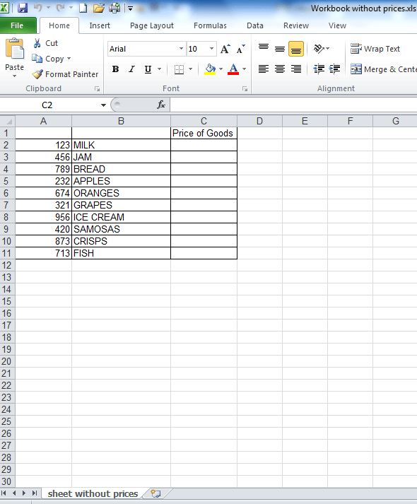
When you open the “workbook without prices” file you will see the screen below. Column C in this workbook is where we will pull in the “Price of the Goods” from the other workbook. Cell C2 in the “workbook without prices” will already be selected – if it isn’t, click in cell C2, as that’s where we want the first result to appear.
Step 2
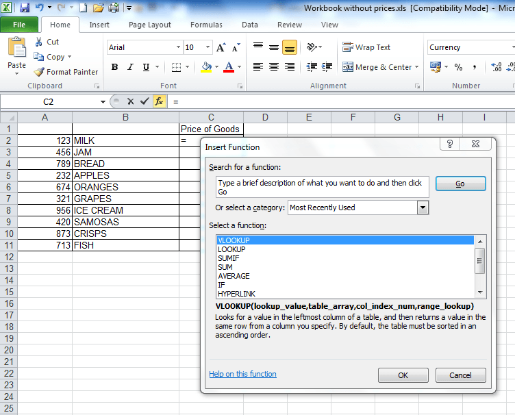
Click on the “fx” button which is just above column B (see screenshot below). The ‘Insert Function’ window will then show up (also shown in the screenshot below). If the “vlookup function” is already selected, like in the screenshot below, click “ok”.
If the “vlookup function isn’t already selected, then in the “or select a category” field shown in the screenshot above, change the option in the drop-down from “most recently used” to “All” then scroll down until you get to the vlookup function, as shown in the screenshot below.
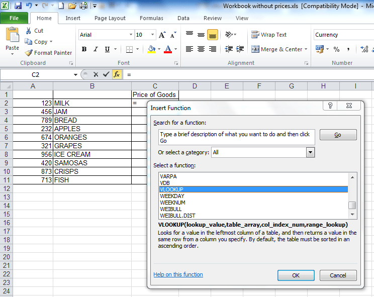
Once you’ve selected the “vlookup function” from the drop down menu and clicked ok, the “Function Arguments” window will appear.
Step 3
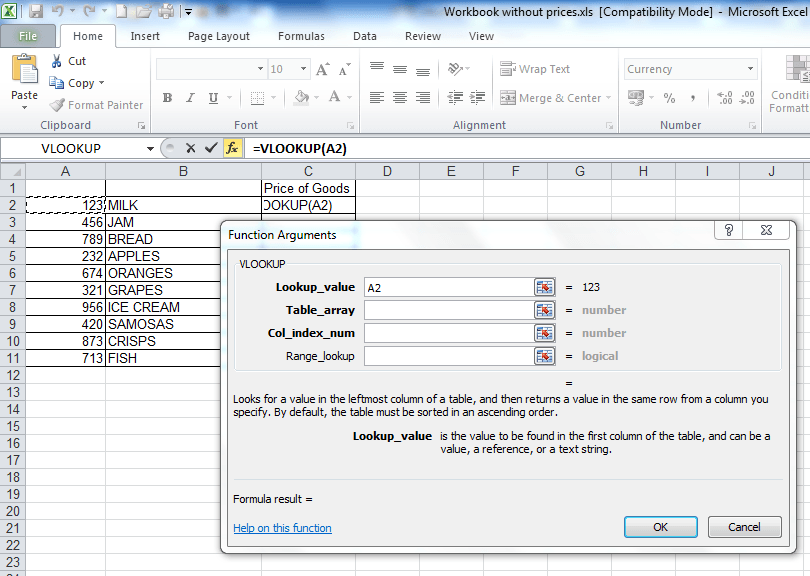
The “Function Arguments” window will show 4 different fields which need to be populated for the vlookup to work. For the first field, the “Lookup_value”, click on cell A2, as illustrated in the image below.
Step 4
Now click into the “Table_array” field (a “table array” is a fancy phrase for describing two or more columns of data).
Step 5
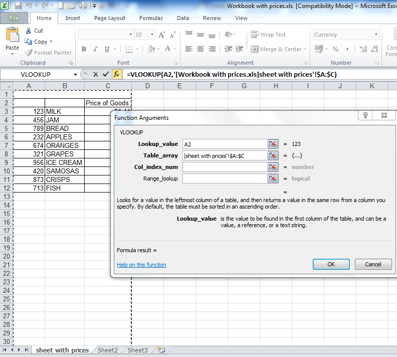
This part is where the other workbook comes in! After you’ve clicked in the “Table_array” field, click into the other workbook (it’s called “workbook with prices”) and highlight columns A – C in that workbook. We highlight columns A – C in this workbook because column A has the “Lookup_value” that is in the “workbook without prices” and column C has the “Price of Goods” data that we want to extract from this workbook. When you highlighted columns A – C, you may have noticed that the characters “3C” appeared at the top of column D – this is a quick way of Excel telling you how many columns there are in the data you’ve highlighted – it saves you having to count the columns manually, which a lot of people in offices do! If you didn’t notice that, clear the data in the “table array” field and highlight columns A – C again in the “workbook with prices” – ensure you hold the mouse key as as soon as you let go, the “3C” will disappear. Many office workers don’t know this trick and waste a lot of time manually counting the columns! But we’re here to save you time!
NB – an alternative, but IMPORTANT way to populate the “Table_array” field is to highlight the range of data you’re looking up, starting with your first unique value – in this case cell A3. So you’d highlight cells A3 to C12, because C12 is the last cell in the range. You’d then need to FIX this table array by putting dollar signs in before the H, before the 2, before the J and before the 11, so your formula at the end looks like this: =VLOOKUP(B2,$A$3:$C$12,3,FALSE). If you’re in the table array field and you press F4, then Excel will do this automatically for you.This is useful to know if a spreadsheet at work doesn’t allow you to highlight columns A to C because some cells are merged or you’re getting an invalid error. But for now, just leave it, ensure, you’re fields look the same as those in the screenshot below then proceed to Step 6, the second last step.
Step 6
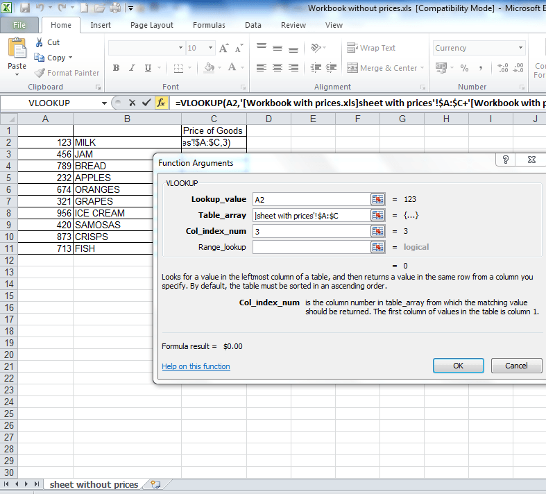
Click into the “Col_index_num” field – you will notice that your screen returns back to the first file, the “workbook without prices” – don’t panic! All you have to do here is put in the number 3. We put in the number 3 here because column C in the “workbook with prices” has the prices of the goods that we want and it is three columns away from column A, which has the unique lookup values that we are using. Or if you noticed the “3C”, it means “3 columns” so you know you have to insert the number 3 in the “Col_index_num” field. A screenshot of how everything should look so far is below.
Step 7
The final step! Click into the ‘range lookup field’ and type the word ‘FALSE’. Click ‘OK’ and, like magic, the formula will return the first result that we’re looking up. After that, simply drag down the formula in cell C2 in the “workbook without prices” and the “prices” of all the other goods in this file will auto-populate. Easy, right!? Typing the word ‘FALSE’ here will ensure that the vlookup only returns an EXACT match. If it doesn’t find an exact match for the ‘lookup value’ we’re using, then it will return an N/A – more about this in the “10 common problems” page above.
Your formula in the end should look like this (in cell C2 in the workbook without prices): =VLOOKUP(A2,'[Workbook-with-prices.xls]Sheet1′!$A:$C,3,FALSE)
If your formula does not look like this, then you need to check that you’ve followed the steps above correctly.
3 people said they couldn’t get to the second workbook in step 5. This is because they hadn’t clicked on the ‘enable editing’ button shown in the screenshots at the beginning of this tutorial in BOTH workbooks! Please make sure you do this if this problem applied to you, before posting a comment. In fact, you should ALWAYS click ‘enable editing’ if you’re using formulas in Excel. It’s good practise and will help you.
If you want to learn about Pivot Tables, you can do so via this website we created following user demand: http://pivottablesinexcel.com/
If you have problems with your vlookup click here – 13 common problems:
We ask that you take a moment to read our Terms and Conditions and Privacy Policies.

This tutorial was quite insightful indeed, thank you.
You’re welcome! Thanks for the feedback. And let me know if you have any questions.
Hi
is it work for two excel work sheets one from desktop another from ondrive
Hi
Yes, so long as you open both files in Excel and save them after you have done the vlookup.
Let me know if you have any other questions.
Thanks
Analyst
Hello Analyst,
What if i want to the output of the Vlookups to be blank if nothing is found, how do I execute please? Instead of having zeros (0) or N/A for missing data, I want the cell to stay empty.
Thank you
Hi Peter
Thanks for your question.
It’s quite easy – I cover how to make the output return a 0, if nothing is found in problem number 10 on this page: https://howtovlookupinexcel.com/13-common-problems-with-vlookups/
So you can just subsitute the 0 with two inverted commas ie “” in the example I’ve given. Then apply that method to your problem.
Let me know if you want me to clarify things further.
Analyst
Really found this helpful. Thank you.
No problem. You’re welcome!
Let me know if you have any other vlookup-related questions.
Analyst
Thank you so much. It has been so easier now. Thanx again & always.
No problem!
You’re most welcome!
This is great value!
Thanks.
Thanks for the feedback – we really appreciate it!
Have a good day!
Great and simple tutorial, for both the single and multiple workbooks. The details were explained clearly and helped me to learn a new skill in no time. Also, including the files to work with was a HUGE PLUS, as the best way to learn this is by doing. Thanks again!
Awesome!
That’s great to hear. Thanks for the feedback and let us know if you have any questions.
Hello, thanks for the tutorial.
I have done vlookup on my data between 2 sheets using ‘name’ as a Look up Value. But when i used ‘identification no.’ as a Look up Value, the result is #N/A. Any idea why I can’t use ‘identification no.’ column? I’ve set both column as numbers format but still it doesn’t work.
Please help me out as I wanna use numbers column in this vlookup rather than the name column.
Hi
Were you using the file available on this site?
If so, can you send me the file, so that I can see what you did?
Hello
Just wanna check, did you received my file? I’ve send it through the email that you replied.
Have a good day!
Hi
Apologies for the delay.
Yes, Ive got the file.
I’ll send it back to you now with the solution.
Analyst
Hi
Thanks a lot for the well explained solution. It’s really helpful and useful. It makes my job easier.
You have made my day!
No problem. If you have any other questions, let me know.
Very well explained, unlike other guides! Thanks!
Thanks J – we appreciate the feedback!
Hi,
i am using VLookup for our company records(product wise against Store). When i am copying details from 1 excel file to another using formula & save it and when i move to another store, the earlier saved data is missing and only the later data is visible. Please advise.
Kind regards,
Vaishu.
Hi Vaishu
I’ve never heard of this problem before.
If the file does NOT contain any confidential data, send it to the email address that you get this response from, and I can have a look.
Analyst
i don’t know what happend i pasted the formula exact as per your advise but still the result was #n/a
=vlookup(a1,[file_name.xlsx]sheet1!$a$1,$c$865,3,false)
kindly advise the appropriate steps for me.
Hi
It sounds like the data in your file is not arranged in the same way as the data in my file.
If the data in your file is NOT confidential, then send it through, and I’ll have a look for you.
Analyst.
Looking forward to learn more new things in vlookup and Hlookup also.
Life changing and work made easy. God bless you for the knowledge shared.
Thank you.
Hello good day! I found it helpful for me but I just want to ask a help for you. I’m really confuse what code/ statement should I use.? The sheet that I created is composed of different kind of places and that places is also composed of results; positive and negative results. I really wanted to easily find and easily count the total number of positive and negative if I just only type the name of the place on the specific cell and to the another cell is the word positive/ negative. What statement/ code should I use? please help me on this. Thank You.
Hi
It sounds like you need a countif formula.
But to understand your problem, can you describe a basic example of what it is?
Eg I assume you have three columns: place, positive, negative then you have the places and whether or not a place is positive or negative in the positive and negative columns?
A bit more clarification is needed.
Analyst
Thanks for the tutorial, can you explain why column B isn’t used as the Look up value?
Hi
You can use column B to do the vlookup, but I’d recommend that you always use numbers rather than words to do vlookups, as you’re less likely to encounter errors if you’re using numbers.
Words may be spelt incorrectly in another part of the workbook, which would cause your vlookup to fail.
Any other questions, just shout.
Analyst
What if I want to pull multiple columns of data to another spreadsheet?
I’d recommend doing vlookups for the columns that you want.
Very well explained.
I have a doubt here. Can you tell me what are the things that we should keep in mind when vlookup is done in single sheet AND with different sheets AND different workbooks?
Thank you so much in advance.
Hi Neethu
The differences between a single sheet and different workbooks are covered in the examples I’ve explained in the tutorials here (singe sheet): https://howtovlookupinexcel.com/ and here (two workbooks): https://howtovlookupinexcel.com/vlookup-between-two-workbooks/
It should only take around 5 mins to go through each tutorial and will be a lot easier than re-explaining everything in the comments here.
With different worksheets, you just click on the different tabs withinin a workbook, instead of different workbooks when you’re doing the vlookup.
I hope that helps.
Analyst