Vlookup between two workbooks / Vlookup between multiple worksheets
Below is an example of a vlookup between two different workbooks, which a lot of you have been asking about.
To make it as easy as possible for you to understand the steps, we’ve included the two files we use for this free excel vlookup tutorial here: Workbook without prices and Workbook with prices.
You can’t learn how to drive a car by just reading a book, and for that reason, we’ve given you access to the files that we use – after all, the best way to learn is by doing! Other sites do not offer you the files, but we do. We recommend that you have both files open before you begin the tutorial.
The workbooks contain a list of products which the majority of people would buy in a supermarket – Milk, Bread, Jam, etc.
We have intentionally kept the files simple. We’re going to use the vlookup function to get the prices of the food data from the “workbook with prices” into the “workbook without prices”.
Step 1
Before you start, open both workbooks from this site AND make sure you’ve clicked the “Enable editing” button in BOTH workbooks then save them to your Desktop, otherwise any changes you make won’t work!
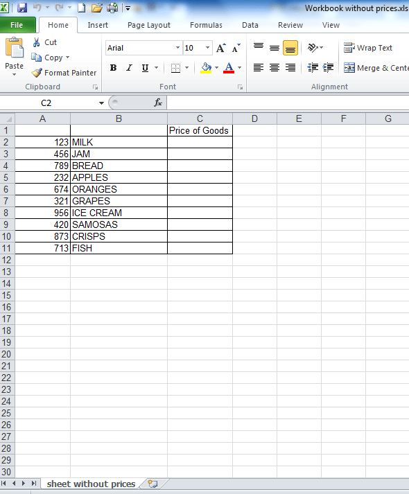
When you open the “workbook without prices” file you will see the screen below. Column C in this workbook is where we will pull in the “Price of the Goods” from the other workbook. Cell C2 in the “workbook without prices” will already be selected – if it isn’t, click in cell C2, as that’s where we want the first result to appear.
Step 2
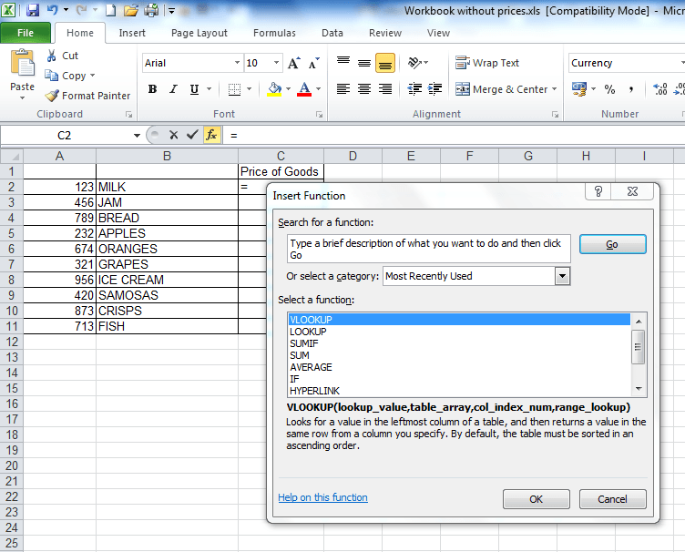
Click on the “fx” button which is just above column B (see screenshot below). The ‘Insert Function’ window will then show up (also shown in the screenshot below). If the “vlookup function” is already selected, like in the screenshot below, click “ok”.
If the “vlookup function isn’t already selected, then in the “or select a category” field shown in the screenshot above, change the option in the drop-down from “most recently used” to “All” then scroll down until you get to the vlookup function, as shown in the screenshot below.
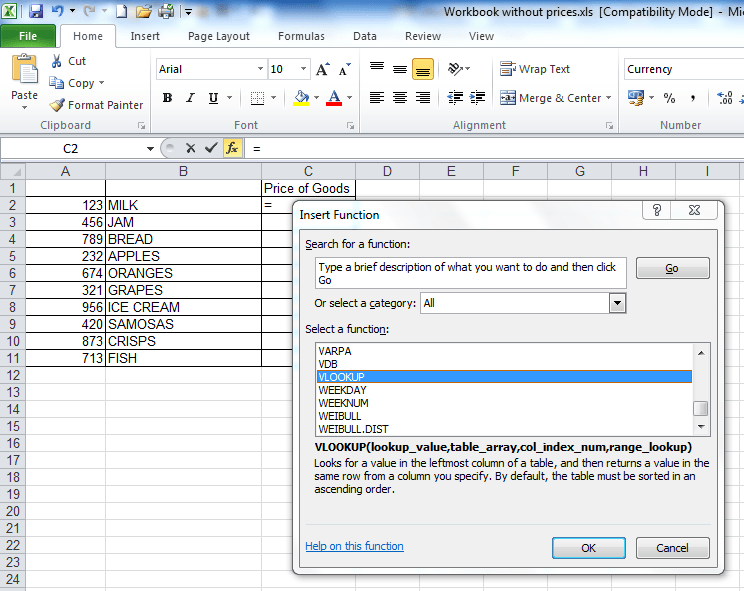
Once you’ve selected the “vlookup function” from the drop down menu and clicked ok, the “Function Arguments” window will appear.
Step 3
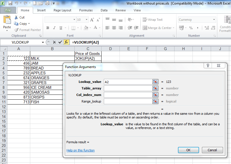
The “Function Arguments” window will show 4 different fields which need to be populated for the vlookup to work. For the first field, the “Lookup_value”, click on cell A2, as illustrated in the image below.
Step 4
Now click into the “Table_array” field (a “table array” is a fancy phrase for describing two or more columns of data).
Step 5
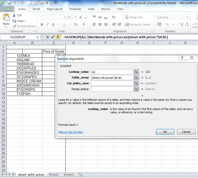
This part is where the other workbook comes in! After you’ve clicked in the “Table_array” field, click into the other workbook (it’s called “workbook with prices”) and highlight columns A – C in that workbook. We highlight columns A – C in this workbook because column A has the “Lookup_value” that is in the “workbook without prices” and column C has the “Price of Goods” data that we want to extract from this workbook. When you highlighted columns A – C, you may have noticed that the characters “3C” appeared at the top of column D – this is a quick way of Excel telling you how many columns there are in the data you’ve highlighted – it saves you having to count the columns manually, which a lot of people in offices do! If you didn’t notice that, clear the data in the “table array” field and highlight columns A – C again in the “workbook with prices” – ensure you hold the mouse key as as soon as you let go, the “3C” will disappear. Many office workers don’t know this trick and waste a lot of time manually counting the columns! But we’re here to save you time!
NB – an alternative, but IMPORTANT way to populate the “Table_array” field is to highlight the range of data you’re looking up, starting with your first unique value – in this case cell A3. So you’d highlight cells A3 to C12, because C12 is the last cell in the range. You’d then need to FIX this table array by putting dollar signs in before the H, before the 2, before the J and before the 11, so your formula at the end looks like this: =VLOOKUP(B2,$A$3:$C$12,3,FALSE). If you’re in the table array field and you press F4, then Excel will do this automatically for you.This is useful to know if a spreadsheet at work doesn’t allow you to highlight columns A to C because some cells are merged or you’re getting an invalid error. But for now, just leave it, ensure, you’re fields look the same as those in the screenshot below then proceed to Step 6, the second last step.
Step 6
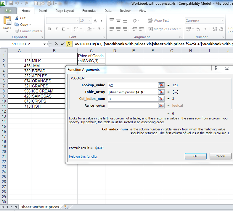
Click into the “Col_index_num” field – you will notice that your screen returns back to the first file, the “workbook without prices” – don’t panic! All you have to do here is put in the number 3. We put in the number 3 here because column C in the “workbook with prices” has the prices of the goods that we want and it is three columns away from column A, which has the unique lookup values that we are using. Or if you noticed the “3C”, it means “3 columns” so you know you have to insert the number 3 in the “Col_index_num” field. A screenshot of how everything should look so far is below.
Step 7
The final step! Click into the ‘range lookup field’ and type the word ‘FALSE’. Click ‘OK’ and, like magic, the formula will return the first result that we’re looking up. After that, simply drag down the formula in cell C2 in the “workbook without prices” and the “prices” of all the other goods in this file will auto-populate. Easy, right!? Typing the word ‘FALSE’ here will ensure that the vlookup only returns an EXACT match. If it doesn’t find an exact match for the ‘lookup value’ we’re using, then it will return an N/A – more about this in the “10 common problems” page above.
Your formula in the end should look like this (in cell C2 in the workbook without prices): =VLOOKUP(A2,'[Workbook-with-prices.xls]Sheet1′!$A:$C,3,FALSE)
If your formula does not look like this, then you need to check that you’ve followed the steps above correctly.
3 people said they couldn’t get to the second workbook in step 5. This is because they hadn’t clicked on the ‘enable editing’ button shown in the screenshots at the beginning of this tutorial in BOTH workbooks! Please make sure you do this if this problem applied to you, before posting a comment. In fact, you should ALWAYS click ‘enable editing’ if you’re using formulas in Excel. It’s good practise and will help you.
If you want to learn about Pivot Tables, you can do so via this website we created following user demand: http://pivottablesinexcel.com/
If you have problems with your vlookup click here – 13 common problems:
We ask that you take a moment to read our Terms and Conditions and Privacy Policies.

the table array isn’t working for me..i have two worksheets – both saved as excel 97-2003. when I click the table array and highlight the columns it wont pick up the information from the other workbook??
Hi
It sounds like you have merged cells in your file.
Have you tried the alternative way described in Step 5? I’ve pasted the comments below, for your convenience.
“NB – an alternative, but IMPORTANT way to populate the “Table_array” field is to highlight the range of data you’re looking up, starting with your first unique value – in this case cell A3. So you’d highlight cells A3 to C12, because C12 is the last cell in the range. You’d then need to FIX this table array by putting dollar signs in before the H, before the 2, before the J and before the 11, so your formula at the end looks like this: =VLOOKUP(B2,$A$3:$C$12,3,FALSE). If you’re in the table array field and you press F4, then Excel will do this automatically for you.This is useful to know if a spreadsheet at work doesn’t allow you to highlight columns A to C because some cells are merged or you’re getting an invalid error.”
Analyst
Nice explanation. Kudoos!!!
Thank you, Sir.
Very neatly explained!
A point to underline, is:
Use $ in table range ensuring the value is looked up throughout the table.
Hi Vishi
Thanks for your comment.
You don’t have to use $ signs to lock the table array if you do the vlookup the way I have explained it in the tutorial.
The method I have shown is the simplest way to do a vlookup and I’ve demonstrated this method, on purpose. However, the alternative of adding in the $ signs is already covered in Step 5.
Regards
Analyst
Great explanation. One issue I could not solve still:
I have ID numbers and names (2 columns of a big sheet containing lots of other columns), and the names column is BEFORE the ID number column I’m searching in…
So: what if the column you want to extract data from is BEFORE the column you use for lookup. Negative ‘column’ offset numbers seem not to work…
Thanks for any pointers.
Hi Peters
If you want to lookup data before then unique ID column, then you’ll need to use a different formula.
But the quickest thing to do would be to just paste the data you’re looking up so that it is AFTER unique ID column.
Let me know if you still have questions.
Analyst
THE FIRST HELPFUL ARTICLE ON VLOOK UP I HAVE COME ACROSS.
THANKS
Awesome! Glad it helped!
Very cool and easy to follow!!! Thanks
Thanks for the feedback, Flick.
Wow! Neatly explained! Thanx alot! 🙂
Thank you.
Thank you for a great tutorial. Certainly useful for old dummies.
You’re welcome.
Hi;
I see that you are an expert in excel functions.
I will appreciate if you can help me and let me know if you have a tutorial to solve vlookup use with 2 sheets with a lot of data. I have experience working with vlookup and pivot tables but I am currently looking for a job and I got a test where the only question was:
Use the “Cash posting” and “Customer list” tab to do vlookup to place customer phone number in the cash posting tab.
Note: both sheets had about 15 columns with aprox 50,000 row of data each.
Thanks for your feedback and hopefully next time I can get this right with not errors in my next job interview/test 😉
I can’t see the “notify me of follow-up comments or subscribe link below in my screen but I wish to receive a response. THnaks again.
Hi
Thanks for your question.
If you go through the tutorial on this page, it will show you how to solve your problem. Doing a vlookup between two sheets is very similar to doing a vlookup between two work books – the only difference is that instead of referring to another workbook in the table array, you’d refer to a different tab in the same workbook.
Let me know if you have any further questions.
Rgds
Analyst
Thank you for this page I have been struggling to vlookup I bumped into this page today and I now know how to look up.
You’re welcome Veronica.
I’m glad the effort to create the site wasn’t in vain.
Hello 🙂
HELP!! If you have a moment, I really need assistance with this one as soon as possible, as I will probably be asked to do this again since I’m covering for the 2 people that normally do this editing.
I just started a contract position with a healthcare company & was asked to compare two (2) excel files [their master directory with the most current information against an affiliates directory with older info.]. These lists contain the physicians name, address, phone, etc. I was asked to make any changes necessary to the affiliates listing. I ended up doing this manually with both files lined up horizontally (well over 1000 rows of data). A LOT of work!
Do you know of an easier way to compare this data for the differences…VLOOKUP or other in EXCEL 2010 or 2013? Please keep in mind that the columns & headers are not exactly the same in both workbooks…formatting is slightly different as well. If you know of an easier way to do this, I would be so VERY GRATEFUL! Thank you. Teresa
Hi Teresa
Yes, there’s a much quicker way to do that!!
The tutorial on this page explains how.
But both files will need to have the same unique identifiers.
eg if you’re looking up data for a particular physician, then their name should appear in both sheets.
If you have unique numbers next to the physicians’ names, then they’ll be the reliable way of looking up the data. I used numbers rather than names in this tutorial.
Let me know if you have any other questions.
Analyst
I spent all day researching this and this is the only website that helped me! Thank you so much! Woooohoooo!
That’s awesome! It’s great when we get testimonials like this! Thank you!!
Hi,
Is it possible to have calculation formulas in the table array for eg where your price column is? I was trying to use IF formulas however this is proving to be too complicated so I opted to try the VLOOKUP. Thank you!
Hi
Absolutely! I look up values in columns with formulas all the time.
If it’s not working, then your IF statement may be written incorrectly.
If your file doesn’t contain any confidential information, then send it through and I’ll have a look.
Analyst
Dude, I never leave reviews however this is the onlyyyyy explanation online that made it work for me…. it has both pictures and descriptions that anyone can use… this is the best really, thumbs up 😉
Andrew
Thanks dude! I appreciate the feedback! I’m glad the time spent putting it together didn’t go to waste!
It is very helpful and it is useful.
Can you please also help in linking the files with Vlookup
Hi Amit
Sorry, I’m not sure what your question is.
Can you re-phrase it?
Analyst
Great explanation, thanks very much.
You’re welcome.
Hi,I have 2 work sheets one work sheets has more than 8000 cols (say sheet 1) and other sheet has 1000 cols (say sheet 2). I have column with Task ID in common but the data is different in both sheets.
I want to compare the task ID of sheet1 with sheet 2 and if matches then I need to return the value of from column ‘Owned by” which is in sheet 2 to sheet 1. Please note that there are more than 10 cols in each sheet and owned by contains duplicates.
Can you please advice how to tackle with this problem,appreciate your kind reply
Hi Sri
Without seeing your spreadsheet, I am not quite clear on exactly what the problem is.
Can you send a file with dummy data to clarify what the problem is?
With the duplicates, I’d strongly recommend removing them, as the vlookup will only return the first ID that it comes across and teh duplicates will also make your spreadsheet larger than it is, especially if it has 8,000 columns.
If you can send dummy date with, say, 3 columns in each tab, I can help further.
Analyst
I have a spreadsheet that I run once a month of incident tickets. What do I need to do step by step to check the newest to the latest to see what tickets have been completed?
Hi
There are a number of ways this could be done.
But you you haven’t clarified exactly how the data changes? I assume the incident numbers are static? And when you run the report, what changes exaclty?
Does an incident description change from “open” to completed”, for example?
If so, you could just put in a column with an IF statement that says “=if(A1=”completed”,”ignore”,”review”) – this would be assuming you have the description of the status of the incidents in column A. This would basically tell you to ignore any incidents that are “complete” and review everything else.
If you can provide more clarity on how the data changes, then we can assist further.
Analyst
i am not able to use vlookup in two different sheets , i need ur help on immediately basis.
pls mail me if you can
thank you so much
Hi
If you send the spreadsheet to the email address that you get this response from, I can have a look.
Please only send it if it does NOT contain any confidential data. Or anonymise it.
Ok, so initially I thought this helped, it worked with my initial set of sample data perfectly. Then when I added more data, it failed. Help? I have a spreadsheet that is used daily, I would like to screen it every day with the new data, to see if a certain list of phone numbers appear, they may appear more than once on any given day, or not at all… Can this work? I’d be happy to email my sample data to show you what I’m trying to do… Thank you.
Hi Danielle
If the sample info isn’t confidential, then send it through and I can have a look.
Analyst
Is it possible to search for data across multiple sheets in a different workbook?
My scenario: I have workbook A which contains a list of ID numbers (A1), I want to search workbook B, which has 50+ tabs which might contain the matching text string from Book A, cell A1, and then bring back some other data. So, go find this ID number somewhere in this other workbook and then bring back the third comlumn which contains a status… is there an easy way to do this?
Hi Nellie
There’s two ways you can do this:
i) create columns in Book A for all the possible columns that you want to lookup data from in Book B, then use the unique ID in column A to look up the data from the different tabs in column B.
ii) copy and paste the data from the different tabs in Book B into ONE single tab in Book B (assuming that the column with the unique ID is always in the same column). So your data from the first tab might cover rows 1 – 49, then data from the second tab might cover rows 50 – 99 in the first tab, and so on.
Let me know if any of the above isn’t clear.
Analyst
Just replied to the email notification I got and attached the spreadsheet. Thanks.
I’ve responded back to you via e-mail.
This helps a lot! Thank you 🙂
You’re welcome, Mary.
Thank you so much! I’m an absolute novice with excel but this is making it much easier to get to grips with.
You’re welcome, Chris.
THANKS for the simple easy to use directions. The real life example REALLY helped understand what I was doing!! THANK YOU!!
You’re welcome, Jen.
Hi Dolly
I’ve updated Step 7 with the following text.
Your formula in the end should look like this (in cell C2 in the workbook without prices): =VLOOKUP(A2,'[Workbook-with-prices.xls]Sheet1′!$A:$C,3,FALSE)
If the formula you have is not the same, then please re-visit the steps, as lots of visitors have managed to get the right results with the same steps.
Wow! Super! I’ve struggled with this for weeks, using two worksheets, and this worked perfect. Life saver for work. Thanks again.
Hi Sheila
That’s great to know! I’m glad the tutorial helped.
Analyst
I just wanted to say how much I like your instructions. They are simple in plain English and easy to follow.
I did the steps you outlined and got it right the first time.
Good job keep up the good work.
thanks
Thank you Rebecca, the feedback is appreciated.
Analyst
Love the way you explain things, in plain “English”. Issue. I have two excel sheets, I’m looking to transfer my “comments” from old one to a new one – weekly.
When I follow these instructions on my new sheet I just get a lot of N/A’s.
Can you assist?
Thank you!!! 🙂
Hi Diana
Are you using numbers, words or characters to do the vlookups?
If you send through 5 lines of anonymised data where you’re getting the N/As, along with anonymised comments, I can have a look.
I have characters and numbers.
Example:
9/2- ST & IN sent to client, call on 10/1.
Hi Diana
If you’re using a mixture of numbers and characters, there is a very high risk of the vlookups not working. In the example you describe, if one sheet had “9/2- ST & IN” but the other sheet had “9/2 – ST & IN” ie a space BEFORE the dash, then you’d get an N/A error straight away!
vlookups are usually done using numbers. Do you have any other unique IDs that you can use instead that consist of numbers only?
If not, if you anonymise 1 row of the data and send me an example of one lookup that has failed, I can tell you what the problem is. Without seeing the file, my first guess would be the issue I’ve described ie inconsistent IDs.
Analyst
Thanks for providing the knowledge…
This was the best and most helpful Vlookup tutorial. I have used MANY tutorials! THANK YOU! You saved an interns life!
Thanks for the feedback, Ashley.
It’s much appreciated.
Hi…your tutorial was great. I need to create a third workbook comprised of data concerning one unique identifier on both spreadsheets. I want all the columns pertaining to the unique identifier from 2 workbooks to appear on the 3rd workbook. Help Please!!!
Hi Lisa
Thanks and apologies for the delay in responding. I’ve been on holiday.
Without seeing your workbooks, I’d have to make some assumptions:
i) you want only pre-populated columns from the two existing workbooks to appear in the the third workbook? If so, this could be done with an IF statement rather than a series of vlookups.
ii) how many unique identifiers are there where you want columns from the existing workbooks to replicated in the third? Or is there a large number that it would be time-consuming to count them?
iii) do the unique identifiers have a common attribute with other unique identifiers in the workbooks es g grades A – C, D – F, etc? Or values under a certain amount?
If you could clarify the answers to these questions, I can assist further.
J
Hi
I have been sent a workbook from a colleague in Spain to complete – I have used vlookup using one of the workbooks on my computer – she has just emailed me to say that when she opens the ‘completed’ workbook my information is not showing?
Hi Aimee
Apologies for the delay in responding. I’ve been on holiday!
I’ve never come across that problem before, but if the data you’re looking up is in one sheet, I’d suggest copying it and pasting it in a blank worksheet within the workbook that you want to do the vlookups in, then send your colleague that file.
Let me know if the suggestion doesn’t make sense and I’ll clarify further.
Analyst.
Thanks alot..very easy and it worked too.
You’re welcome Rekha.
Good morning
Please assist, I want to do a vlookup on a 3 workbooks, I want to look for account numbers that are paid up on the three spreadsheets (October, November and Decemeber).
Thanking you in great anticipartion.
Hi
Without seeing your workbook, I can’t tell you what your formula should look like. But if you read the tutorial on this site, you should be able to grasp the principles of how to do a vlookup very quickly as hundreds of other people have done (from the comments on the tutorial pages). The file in the tutorials is also available to download from this site.
Very easy to understand, thanks a lot. I need to learn mysql, have you published any other site to learn mysql like the way you have explained for vlookup.
Hi Rajesh
No, I don’t use mysql in my job, but thanks for the compliments. Let me know if there are any other things that you want to learn and I’ll post content if I have experience of using them.
have u posted vlookup with more examples.
nd I want to know have u posted any youtube video for vlookup and pivot tables.
Hi
Not yet – an ebook with more examples will be available soon – in the next few weeks.
What is the link to the E-Book?
Very good and informative article. Simple to learn and very informative.
Does this not work if the value im searching for is a text value?
No, I’d recommending changing the format to ‘General’, ‘Number’, ‘Currency’ or any other format.
Hi,
I want to lookup data based on combination of 2 data (ex-search for combination 123 & MILK in the second sheet). Is there a way for that.
Please help
Hi Janani
Apologies for the delay in replying.
Yes, you can do that – the easiest way would be to create a new column summing up the two columns – I’d insert this formula into cell D3 in the workbook with prices: =A3&B3
Drag the formula down to the rest of the cells in that column, then do a vlookup for the data in that column. Let me know if you want further clarification.
Hello
I attempted this D3=A3+B3 and receive the #VALUE! Where did I go wrong?
Hi
I’m assuming you want to combine (rather than add) the values in columns A and B?
If so, the reason it didn’t work is because you used “+” instead of “&”.
You should use A3&B3 – that works.
You can’t add numbers and words – which is why you got the #VALUE error.
Let me know if not clear.
Thank you very much!
I love these tutorials
You’re most welcome. An ebook with more examples will be available soon, in case you’re interested. Let me know.
Yes, very much so. Do you work with any other office applications?? Your format has been very effective in my experience(which has only been a few hours,but I am invested.)
Ok, great. I do use other Office applications, but Excel is the one I’ve used the most!
If there is another application in particular that you have questions on, let me know, and I may be able to help.
Thanks for the feedback though. It’s encouraging! 🙂
Thanks a lot…easily explained
good example. i found it really helpful
One of the best ways of explaining the formula. Awesome.
Thanks
Plain speaking and simple, Brilliant.
Thanks
Thanks.
It was a great help..and very easy to grasp..Thanx…!