We’ve covered more vlookup problems than any other site on the internet. If you’re experiencing an issue, read on for solutions to some of the most common problems with vlookups.
This page assumes you already know how to do a vlookup – if you don’t know how to, click here for the link to the 2007/2010 tutorial or here for the 2003 tutorial. The file with the data for the tutorials is here – once you’ve done a vlookup in col D as explained in the tutorials, you can replicate the problems below, if you wish. Or, alternatively, you can just review the list below to find the problem you are experiencing.
1) vlookup n/a error (because wrong range of data is selected)
Here’s a problem from someone who visited this site (and the solution, of course!)
Rather than use the method described, they’d started by typing “=vlookup….” and had selected an incorrect range of cells to look at.
They said they had doubts about the vlookup function and didn’t know how to use it properly.
They were getting an n/a error and didn’t know why! So I got them to send me the file available on this site to see what they’d done wrong. There were 5 N/A errors in their spreadsheet but I’ve left only one instance of the error in the file, to make it easier for you to understand why it happened.
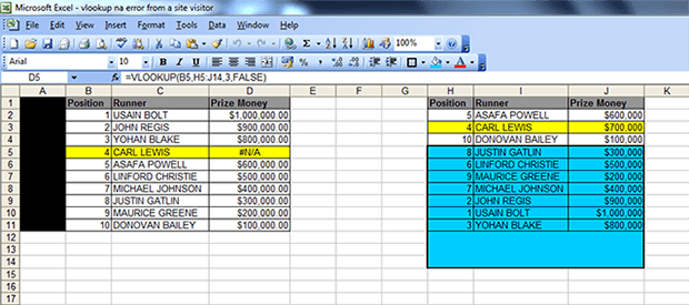
The cell with the N/A error is cell D5 (see screenshot above). It has an “N/A” instead of the value “$700,000”. You can clearly see that Carl Lewis is in position 4 in both tables (left and right); and if you look at the table on the right, the Prize Money assigned to him is $700,000.
Here’s a link to the file with the error, in case you want to see it in closer detail – LINK TO FILE
The non-technical language explanation for this is that their vlookup formula was looking for a result for Carl Lewis in the BLUE AREA, when the result for Carl Lewis is in the YELLOW AREA ie ABOVE the BLUE AREA. (The vlookup was referencing the runner in position 4 but I have used the runner’s name as it’s quicker and easier to understand).
The technical explanation is this: the formula they created in cell D5 was this =VLOOKUP(B5,H5:J14,3,FALSE) where:
B5 is the runner in position 4 in the first table – which is ok (this is the lookup_value)
H5:J14 is the BLUE AREA – which is NOT ok (this is the TABLE ARRAY)
3 is the column reference – which is ok (this is the column_index_number)
FALSE – which is ok (this is called the Range Lookup but it’s simply the last part of the formula to complete the argument and ensure an exact match is returned, and if not found, then an “N/A” is returned.
There are two solutions for this:
either use SOLUTION 1 which is =VLOOKUP(B5,H:J,3,FALSE)
OR use SOLUTION 2 which is: =VLOOKUP(B5,$H$2:$J$11,3,FALSE)
With SOLUTION 1, we are just changing the cell selection for the TABLE ARRAY from H5:J14 to H:J ie take out the numbers! Putting the wrong numbers in the TABLE ARRAY part of the formula will cause an “N/A” error. In this case their formula started at cell H5 (which is position 8) but it is BELOW the area where the result they’re looking for (position 4) which is in the YELLOW AREA.
With SOLUTION 2, we are fixing the range of data from which the formula will search for a result. However, we cover all the “positions”, “runners” and “prize money” in the range. The visitor’s range was missing the $ signs and the cells H2 to J4.
So you can either highlight columns H to J in their entirety, as explained in the tutorials (see step 5 here: https://howtovlookupinexcel.com/) OR – highlight the range of cells of the data you’re referencing.
2) vlookup n/a error (because data is missing from table)
– this will happen either because the data you are looking up doesn’t exist (see table below where the numbers 1, 3 and 5 are not in the second table. You’ll notice that the ‘prize money for the runners in position 1, 3 and 5 in the first table is “N/A” instead of the actual value), so the formula returns an “N/A” instead of the result that you’re looking for.
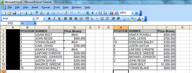
– Or, alternatively, as above, the format of the data in your reference columns is ‘text’. You can fix this in one of two ways:
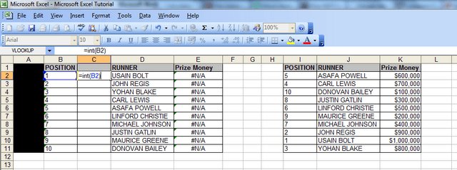
– i) the EASY way is to insert a column after your first reference column (so insert a column in between cells B and C, then type the following formula in cell C2:
=int(B2) then press ‘Enter’ (see screenshot below). After pressing ‘Enter’ drag down the formula so that all the cells in column B are made into ‘integers’ in column C. Now highlight the numbers in column C, copy them, then highlight the cells in column B and click ‘paste Special values’. Now delete column C, and your vlookup will work, like magic!!
– ii) the OTHER way is to change the format of each cell in col B to ‘general’, click ok, then press F2, then press Enter. (NB You must carry out those steps in exactly that order, otherwise they won’t work! Make sure after changing the format of the cell to ‘general’ and clicking ok, that you press F2 BEFORE pressing enter). However, with this method, you would have to do one cell at a time, which is time-consuming. I’m here to save you time!
3) vlookup #REF! error
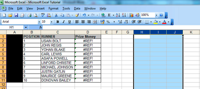
This will happen if the file, spreadsheet or table array that you were looking up data from has been deleted. An example of this is below, where I have deleted columns H to J and the vlookup described in the example above is returning the #REF! error.
4) vlookup not working for some cells/vlookup not working sometimes
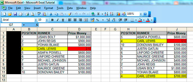
– if this happens, it is usually because your unique value is listed more than once in your reference table. And it would also have different values assigned to it. The screenshot below illustrates what I mean.
– The number “4” appears twice in column H in the table on the right hand side, so the vlookup formula returns the first value assigned to the number “4” in that table, which happens to be $10 (highlighted in red) in column J. If that row was deleted, then the vlookup would return the next value that it found assigned to the number “4” in that table, which would be $700,000 (highlighted in yellow at the bottom). In this example, $10 “Prize Money” is an unlikely amount for any athlete to get paid, as you can see all the other values are much higher, so the vlookup is returning the wrong result. To fix this, you would need to delete any duplicates that are irrelevant in your reference table.
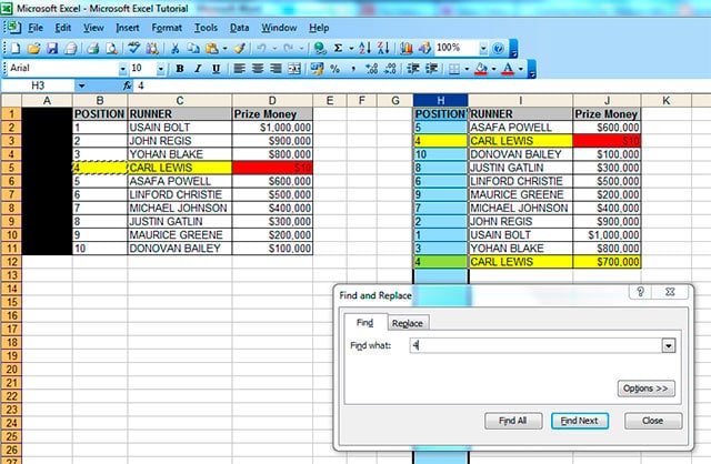
– to find out if a value is a duplicate in a spreadsheet that you’re working on, copy your unique value from your first table, in this case “4” in column B on the left hand side, go to your reference table or the other data that you are looking up (table on the right hand side above) against and press ctrl+f then paste your unique value in the field that comes up shown below. Click on “Find Next” and Excel will move to each row where it can find the number “4” whenever you click “Find Next”. If it appears in the table more than once, then your likely to find that your vlookup is returning the wrong data.
5) vlookup not working – just showing formula.
If your vlookup isn’t working, and is returning the formula like this (see cell D2)
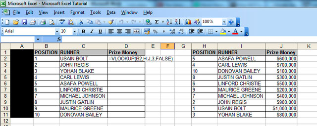
then you need to
– left click into the cell where the formula isn’t working
– right click and choose ‘format cells’
– you will notice that the current format is ‘text’
– change this to ‘general’
– click ok
– then press F2
– the result in the first cell will appear
– now all you need to do is drag that cell down
6) sum of sales data not working because some vlookups are returning N/As:
You may have experienced a problem at work where you are analysing data, and you have a spreadsheet with vlookups and a ‘sum function/total value formula’ at the bottom of each column with the vlookups. However, your sum function may be returning the word “N/A” instead of a total value or an actual figure.
You can fix this by changing your vlookups so that if they don’t find a value, they return a “0” instead of an “N/A”. The sum function will usually not work if there are “N/As” in the column concerned.
I have added in an extra row here (with Donald Trump as runner) to illustrate the above problem.
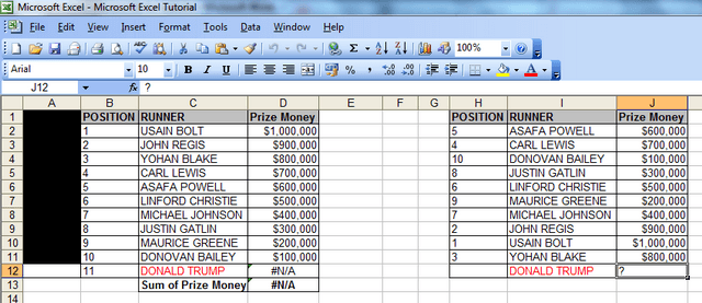
To fix this, you need to add an IF statement to your vlookup. Let’s take the vlookup formula in cell D11 which currently looks like this: =VLOOKUP(B12,H:J,3,FALSE)
If you add the following text, the formula will return a “0” instead of an “NA”, and this will allow the sum function (=SUM(D2:D12)) in cell D13 to work. So just add these bits (I would suggest putting an apostrophe in front and writing this formula in a separate cell first):
i) ‘=IF(ISERROR
ii) copy and paste your original vlookup straight after the above ie (VLOOKUP(A2,I:M,5,FALSE)
iii) add the following ),0,
iv) then paste the original vlookup again (VLOOKUP(A2,I:M,5,FALSE) and add two brackets )) at the end to finish the formula (if you then take out the apostrophe and paste the formula into cell D11, the vlookup will return the value “0” and your sum function//totals formula will work.
v) the revised formula will look like this: =IF(ISERROR(VLOOKUP(A2,I:M,5,FALSE)),0,(VLOOKUP(A2,I:M,5,FALSE)))
The above formula basically says “if there is an error with the vlookup, return the number “0”, and if there isn’t an error, then return the value that the vlookup is looking for.
7) vlookup not working when using a 2007 (or 2010) Excel file and you’re looking up data from an Excel 2003 file (or vice versa).
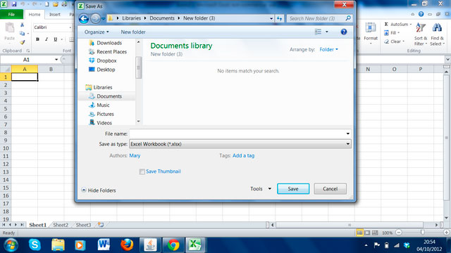
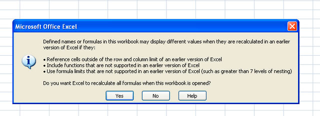
– in the Excel 2007 or 2010 file (s) [NOT 2003], click on ‘file’ then ‘save as’ then in the ‘save as type’ drop down menu at the bottom of the ‘save as’ pop up window, change file type from ‘Excel workbook (*.xlsx)’ – see screenshot below – to ‘Excel 97-2003 Workbook (.xls)’. You will then get the error message shown below in the second screenshot below, at which point, you click ‘yes’. Your vlookup between the files will now work!
8) vlookup invalid error / vlookup invalid reference error
– If you’re working with large spreadsheets, ie those that have over 65,000 rows, you’re likely to come across the “vlookup invalid error” – the “invalid” message appears next to the table array field (see screenshot below). If you complete the vlookup anyway, you’ll then get another error message (see second screenshot below) which says “Invalid reference. This file version can only have formulas that reference cells within a worksheet size of 256 columns (column IW or higher) or 65,000 rows.
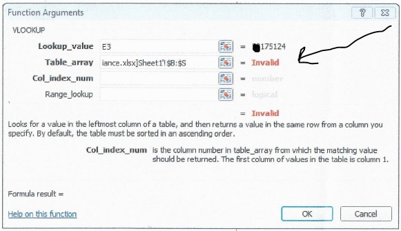

The solution here is two-fold:
i) Ensure that if your table array has more than 65,000 rows, you put anything between rows 65,0001 to 130,000 in a separate sheet, then put anything from rows 130,001 to 195,000 in a separate sheet, and so on, in increments of 65,000, because that’s the maximum number of rows the vlookup function will look it.
ii) Ensure that rather than highlighting the columns (for your table array), you highlight the specific range of cells you’re looking up and “fix them” by pressing F4 – in the example on this site, the specific range for the table array would be cells H2 to J11 – you can see this by either downloading the spreadsheet – available at the top of the site; or simply looking at the screenshot in problem number 5 above.
Hope that’s solved all your problems! Have a nice day!
Hi – very helpful article, thank you. The problem I’m having is odd. I am trying to pull a terms payment description for a long list of accounts. When I enter the formula in row #1, the result is accurate. When I drag (or double-click) the formula to auto-fill the remaining rows, I get the same result as row 1 for the entire data set. I checked the formula in each cell and it is accurate. When I click in the formula and press Enter/Return, the cell changes and shows the results that I want. I don’t have the time to click in each row and press return for the thousands of rows that I need updated and I haven’t been able to resolve the problem. Any ideas?
Thanks in advance!
Onio
Yes – the calculation is set to “manual” in your spreadsheet.
In Excel 2003, go to Tools/Options/Calculation tab then click on “automatic” (you will notice that the “manual” radio button will have been checked but this needs to be changed to “automatic”)
In Excel 2007 or 2010, click the Office button / Excel options / Formulas then select “automatic”.
Thanks for a wonderful tutorial. I’ve been trying for years to master this function but always gave up in frustration so thanks again. I have a question…vlookup will only return one column of results right? Eg. I have a list of employee ids and names and I need to pull in pay increase amounts in one column and the currency code in the next column. Vlookup will only give me the pay increase amount but not the currency code beside it. Is there another function that I should be using?
Hi Carol
Yes – the vlookup will only return one column of results.
I’d suggest putting the currencies in one column (eg column E) putting the pay increases in the adjacent column (eg column F) then using the “&” sign to join the currency and pay increase values.
Eg if you had the “£” sign in cell E1 and a pay increase of 1,000 in cell F1, then in cell G1, you could put in the formula “=E1&F1” which will combine the two fields.
You could then just drag the formula down, assuming columns E and F are populated with the currencies and pay increases, respectively.
Hope that helps – let me know if not.
Rgds
Analyst
i have list of employees by names and professions (Main File).. on other excel sheet i make summery for each profession .. i want to use lookup formula so when i add or remove employee in main list .. then it should automatically change in summery… can you advise how can i manage ..
Hi
If you want a summary table to automatically change, then you should create a pivot table then right click your mouse then click “refresh data” and your summary table will update with all the latest data, assuming that you’re changing it, which you appear to be from what you’ve described.
The tutorial here will show you how to create a pivot table to summarise data: http://pivottablesinexcel.com/
Hi, Great site thank you…
Wonder if you can help me?
I have two spreadsheets open and looking up one ref in another spreadsheet to return a value in the long list there, as I select the range in the second list and highlight the range this does not get entered into the range area for the formula toolbar in the first spreadsheet and when I press enter after selecting the range the cursor just moves one cell down in the selected range and stays on the second spreadsheet, not entering the range and going back to the formula toolbar in the first spreadsheet…
Any suggestions would be appreciated!
Thanks
Stuart
Hi Stuart
I believe this may have happened because there are some merged cells in the second spreadsheet, which are preventing you from highlighting a distinct set of columns eg if some of the column titles in the second spreadsheet span several columns, and the cells where the titles are in have been merged, then that could be the issue.
I’d suggest highlighting the range of cells rather than the columns, so using the screenshot in problem 1 above, instead of highlighting columns H to J for the table array, select the equivalent of cells H2 to H11 with your mouse in your second spreadsheet. If that doesn’t solve your problem, let me know. If you send a file with dummy data I can investigate further if problem not solved.
This article is truely very helpful
Hi this is Prasun. I had no idea about excel vlookup. This post helped me to learn about vlookup. Thank you very much sir.
You’re welcome.
how to match a sheet1 from sheet2 by applying vlookup, and if a number given in sheet1, how to apply to sheet2, means match the number by two sheet. pls suggest. thanks
The answer to that question is here: https://howtovlookupinexcel.com/vlookup-between-two-workbooks
Hi,
I have a problem when using emails as the lookup value. I just have emails as the unique text in the sheet and I need to get data from one sheet into the other. The result is #N/A.
What can I do?
Hi Jonathan
It’s a bit risky with emails, as if you have “jonathan@gmail.com” in one sheet but “jonathan@gmail.com ” in the other sheet ie the latter has a space at the end, then the lookup won’t work as the characters don’t match because one unique value has a space at the end and the other one doesn’t. If you don’t believe me, add this formula to cell D2 in the specimen files I’ve provided at the top of this page: =VLOOKUP(C2,I:J,2,FALSE) then edit cell I10 by adding a space at the end. You will notice that the value of $1,000,000 in cell has now changed to an “N/A”
I have a problem with Vlookup. I’m able to match 2 files for some common service tag (alpha numberic form). some come back as NA though. However when I did a search for those NA tags in the file i’m able to find it. My question why is the lookup only able to match for some and not all.
I have tried #1 and #4 but it’s not working
Hi Asmaa
If you’ve done it correctly, then the only other thing I can assume that could be wrong is that the last bit of the formula is missing ie the word “false” is missing from the “range_lookup” field. However, without being able to see your file, it would be a bit like a car mechanic guessing what a problem is without looking at the car. Let me know if the suggested solution works.
Thank you so much for this. My problem was #4. Sometimes the obvious is right in front of you and you still can’t see it.
No worries – glad I could help!
I found the solución! I forgot to lock my array! I am sorry about the trouble. Thanks for a great forum though
No worries – glad you resolved the problem!
SCENARIO: I have one document with two different tabs. The first tab has a table with store numbers and the full address of each store. The second tab had the store numbers and which products are sold in each store. I need to add a column in the second tab which shows the city for each store (found in tab 1). I am using a vlookup formula. It does work!
FORMULA USED =vlookup(A2,Tab1!A5:G1972,7,FALSE)
PROBLEM: When I try to copy$paste the formula down the entire column it works only for about 80% of the cells. The rest of the cells show n/a. I then have to input the formula again in those n/a cells for it to generate the cities.
QUESTION: Why am I unable to copy&paste the formula down the entire column without some cells being ´´forgotten´´?
Thanks in advance!
Vlookup for text does not work ?
Do you mean a vlookup with words in general or are you referring to this article?
Hi,
I’m really struggling with a VLOOKUP. I’ve used the suggestions above but still can’t get the VLOOKUP to work. I’m trying to get the VLOOKUP to return supplier names against products. The VLOOKUP is returning supplier names that are not linked to the products. Any thoughts would be greatly appreciated.
Hi Katy
If you’ve done the vlookup correctly, then the only reason it would return the wrong suppliers in some instances is because the ‘table array’ or ‘data that you’re looking up’ has more than one supplier assigned to a product. So if you had a product with the number 7456, it may have Nestle and Pepsi Co, for example listed against it, because Pepsi Co was an old supplier and Nestle is the new one. Additionally, some products may be dual supplied, so there’d be two different suppliers listed against them. I’d suggest using ‘ctrl+f’ to search for a product with an incorrect result to see how many times it comes up in the data you’re looking up – if more than once, it most likely has two or more suppliers listed against it.
When I am in the table array box and click on the worksheet that I want data looked up (it is a separate document) the table array box goes away and does not recognize the worksheet I need to look up data in. What could be wrong? Thank you!
Hi Marie
Apologies for the delay – I’d need to be able to replicate the problem you’re experiencing, in order to advise on a solution. Can you send a file with perhaps two rows of dummy data from each tab? info@howtovlookupinexcel.com
Help, please! I’ve got 2 large spreadsheets that have employee names (and ssn) listed. One list is the master employee list and another is an hour upload which includes some employees that are not on the original list. I’ve done a lookup where I’ve used column A on the master EE list as my lookup table then I tell it to use the column on the 2nd table which includes employee ssn there to match those up. The hour upload (the 2nd table) contains lots of duplicates so there are tons of files. When I provide the array (A2:A1406), it tells me that ‘not enough arguments were entered for this function’. Then, when I try to run it, I get a #Name error. Any ideas what I’m doing wrong? Thanks!!!
Hi Jordan
If it says that there are not enough arguments entered for the function, then a part (or parts) of your formula may be missing.
Have you ensured each part when you’re doing the formula is covered as per the tutorial? The different parts are below – I guess you may be missing one of the last parts?
=vlookup(lookup_value, table_array, col_index_num, range_lookup)
Without looking at the file, it’s difficult to advise.
I am having the same issues as Moina #4, my options are set to automatic but I am still getting the same problem, can you help?
Hi Sam
Without seeing he file that you’re using, I can’t diagnose the problem. The manual / auto solution always works for me in instances like these. If you wish, I can contact you directly via email to resolve this. Let me know if you wish to take this route.
I have a vlookup formula that has numbers and alpha involved is that why my vlookup is not working? Because it brings back a value of “0” instead of “5TPABULK”
Hi Kris
I experienced a similar problem today.
It’s probably because “5TPABULK” is missing in the data that you’re looking up. I’d suggest you go to your table array / spreadsheet you’re looking up data from and press ‘ctrl’ and ‘F’ at the same time then put in 5TPABULK in the ‘find’ box to see if it is actually there. If it isn’t, then the vlookup will return a “0”.
Hi, i’m a student and we just started with excell vlookups, and thus far your tutorial has been helpfull, but i’m having difficulties on vlookups with if functions.
Hi Vincent
What are you trying to do with the IF functions? The most common use for IF functions is covered in problem number 5 on this page of the site: https://howtovlookupinexcel.com/6-common-problems-with-vlookups
Hi, I am doing a vlookup and it works fine in some cells, but gives me #N/A in other cells for the same codes (medical cpt codes). I verified that the codes I’m looking for are only listed once in the table array. Do you know why this is happening?
Hi Veronica
#N/As usually appear if the lookup values don’t exist in the data or table array that you’re doing a vlookup from. However, if you have verified that the data exists, then the other problem could be the formatting. I’d suggest you trying either solution (i) or (ii) in point 1 – vlookup #N/A error on the 6 common problems page.
Fabulous! Item #4 solved my issue which has plagued me on several occasions over the last few years. This is great to know – I knew the Lookup data needed to be in a ‘General’ format, but didn’t realize the formula cell itself had a format which was ‘Text’. Once I changed it to General as well, it worked… well, and using the F2. Thank you so much!
Glad I could help!
I have two sets of data for a simulation, one where the time goes up by 0.01 seconds each row and the other where the time goes up by 0.1 seconds each row. I want to put the data for the 0.1 seconds next to the same time for the 0.01 seconds – so I am looking up based on time.
If I put “false” in the last variable, I get all #N/A’s. If I don’t, then I get the right number, but it starts one row down from where it should. How can I fix this?
Submitted on 2013/07/29 at 10:11 pm | In reply to Honelicious.
Hi Erin
Without seeing the spreadsheet itself, it can be difficult to advise on excatly what you need to do. If you would like to send me the spreadsheet via the ‘Get your problem solved for $7’ section on the website, I can fix the problem for a fixed fee of $7 – this will include reviewing your spreadsheet for anything that may not make the vlookup work, as well as writing out the steps that I took to fix the problem. Let me know if you’d like me to do so.
Problem-1sir i would like to know how we use vlookup when we r combining sheet1 to another sheet 1.
Problem-2 Sir i would like to know what is the way to update list in data validation.i have put five names & validate it.2 r 3 minutes 2 r 3 name i have mentioned.but it is not coming in data validation what process.
The principle’s the same – if sheet 2 contained the data in columns H – J in my example, then when you click into the ‘table array’ field in Step 4 in my tutorial, you would click on sheet 2 and then highlight the equivalent of columns H – J in sheet 2, type the column index number (in this case 3 in step 6) then type the word false. I will look into doing a vlookup between two workbooks in future.
The problem I’m having with vlookup is that it’s returning N/A – but only when the number ends in .3333 or .83333 etc – only iterations of repeating 3s. If I go through and change each cell to general, ok, f2, enter, it returns the correct data. But I have A LOT of data and going through each cell is not plausible. Do you have any suggestions?
Hi Jade
Could you provide a bit more detail on the problem you’re having?
I assume you’re using a spreadsheet of your own? If so, are you able to send one row of data as an example? Or, you could simply paste an example of the numbers you are using as the reference point eg cell B2 in my examples, as well as the numbers you are trying to look up eg cell J2 in the examples above. Also need to know current format of the cells in your sheet (right click on one cell with the data, then click format cells).
I’d need to know
The only issue I have with the VLOOKUP is that the formula doesn’t stay the same in all the cells, it gives me the result I’m seeking; however, the numbers change and so forth from point A to point Z in array of 847 entries, but when I put the original formula back in any specific cell, the formula has no issue operating correctly, I’m confused as to how and why this happens, can you explain, thanks!
Hi Carlos
You probably have several different results for each value that you’re looking up – see problem number 3 on the “6 common problems…” page. Let me know if that doesn’t solve your problem.