We’ve covered more vlookup problems than any other site on the internet
vlookup #N/A error? There are FIVE different #N/A errors and two different #REF errors explained below, as well as others such as the “Invalid reference” error. If you experience a different #N/A or #REF error to the ones listed below, then tell us. We’ve discovered new errors as a result of engaging with site visitors. But please check the solutions listed below first!
This page assumes you already know how to do a vlookup – if you don’t know how to, click here for the link to the 2007/2010/2013/2016 tutorial or here for the 2003 tutorial. The file with the data for the tutorials is here – once you’ve done a vlookup in column D as explained in the tutorials, you can replicate the problems below, if you wish. You can also just review the list below to find the problem you are experiencing.
- vlookup number stored as text (#N/A error)
- vlookup trailing spaces error AKA “the invisible dash!” (another #N/A error)
- vlookup #N/A error (because wrong range of data is selected)
- vlookup #N/A error (because data is missing from table)
- vlookup #N/A error because wrong ‘lookup value’ is used in the formula
- vlookup #REF! error because data is missing
- vlookup #REF error because table array is incorrect
- vlookup working for some cells but not others
- vlookup not working – just showing formula.
- Sum of sales data not working because some vlookups are returning N/As
- #NAME error – because of incomplete ‘argument’ in the formula
- vlookup not working when using a 2007 (or 2010) Excel file and you’re looking up data from an Excel 2003 file (or vice versa).
- vlookup invalid error / vlookup invalid reference error
1) vlookup number stored as text (#N/A error)
This is a formatting error that is very easy to fix!
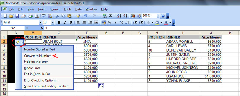
If you get an “N/A#” error and there is an exclamation mark next to the unique value used for your vlookup (see cell B2 in the screenshot below) then you simply have to click on the exclamation mark box the click on “Convert to Number.”
This will change the format of the cell from “Text” to “Number” and the vlookup should work. If it still doesn’t work, read on for other N/A errors covered on this page.
2) vlookup trailing spaces error AKA “the invisible dash!” (another #N/A error)
Some company reporting systems automatically generate reports where each unique value in the report has a trailing space at the end, which causes the vlookup to fail. This is the most difficult “N/A#” error to spot if you’ve never come across it before, as everything “appears” to be normal to the naked eye!
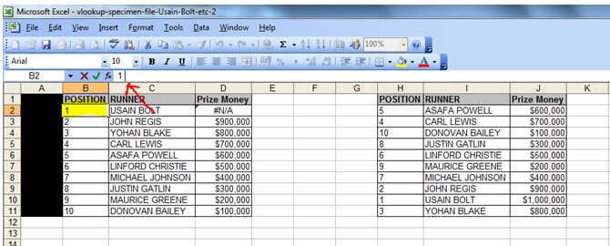
The unique values in the table below are in column B (the positions of the runners). I’ve highlighted cell B2, which has the runner in position 1 – in the toolbar, where the number “1” is shown ABOVE column C, there is a trailing space at the end (see red arrow) which caused the vlookup to fail and create an “N/A#” error in column D.
There are a number of solutions for this:
2a) the “Data – ‘Text to Columns’” solution.
Go to “Data” in the tool bar, then click on the “Data” tab (it’s in between the “Formulas” and “Review” tabs).

Now – and this is an important step – highlight the column where your lookup values are. In the main example on this site, the lookup values are in column B.
Then click on the “Text to Columns” icon in the tool bar.
![]()
Click “Next” in the window that pops up (make sure you leave “Delimited” as the file type).
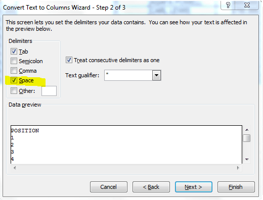
Click on the “Space” checkbox in the next window (see screenshot below). The “Treat consecutive delimiters as one” checkbox will automatically get ticket when you click on the “Space” checkbox. That is fine. Just click “Next” in the screenshot below. Then click on “Finish” and that’s it!
2b) take out the trailing space by clicking in the cell and pressing “backspace” at the end of the cell, to remove the blank space. However, this is time-consuming.
2c) click on the exclamation mark next to the cell then click “convert to number” – this is good, but it also a time-consuming solution.
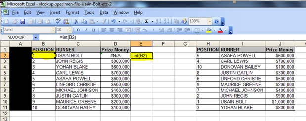
2d) Use the “=int” formula as demonstrated in the screenshot below – using a blank column, enter the formula “=int(” then cell number that you need to fix, in this case, cell B2, then close the brackets – the complete formula will look like this
=int(B2)
Now double-click the bottom right hand-corner of this cell so that the formula is dragged down and then copy the column from the cell where you first entered the”=int()” formula in this screenshot this is cell E2; and then click cell B2 (the cell that needs to be fixed) and then click file / paste special / values – this will convert all the cells in column B to “integers” and at the same time remove the trailing spaces. Voila!
3) vlookup #N/A error (because wrong range of data is selected)
Here’s a problem from someone who visited this site (and the solution, of course!)
Rather than use the method described, they’d started by typing “=vlookup….” and had selected an incorrect range of cells to look at.
They said they had doubts about the vlookup function and didn’t know how to use it properly.
They were getting an n/a error and didn’t know why! So I got them to send me the file available on this site to see what they’d done wrong. There were 5 N/A errors in their spreadsheet but I’ve left only one instance of the error in the file, to make it easier for you to understand why it happened.
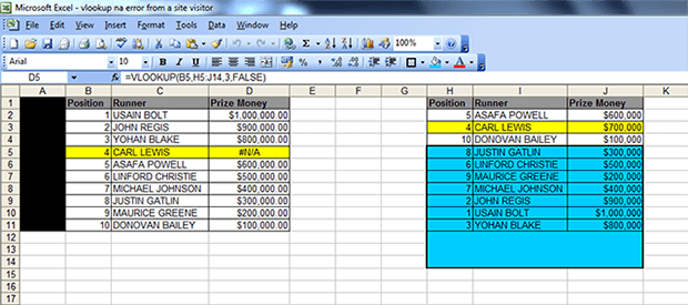
The cell with the N/A error is cell D5 (see screenshot above). It has an “N/A” instead of the value “$700,000”. You can clearly see that Carl Lewis is in position 4 in both tables (left and right); and if you look at the table on the right, the Prize Money assigned to him is $700,000.
Here’s a link to the file with the error, in case you want to see it in closer detail – LINK TO FILE
The non-technical language explanation for this is that their vlookup formula was looking for a result for Carl Lewis in the BLUE AREA, when the result for Carl Lewis is in the YELLOW AREA ie ABOVE the BLUE AREA. (The vlookup was referencing the runner in position 4 but I have used the runner’s name as it’s quicker and easier to understand).
The technical explanation is this: the formula they created in cell D5 was this =VLOOKUP(B5,H5:J14,3,FALSE) where:
B5 is the runner in position 4 in the first table – which is ok (this is the lookup_value)
H5:J14 is the BLUE AREA – which is NOT ok (this is the TABLE ARRAY)
3 is the column reference – which is ok (this is the column_index_number)
FALSE – which is ok (this is called the Range Lookup but it’s simply the last part of the formula to complete the argument and ensure an exact match is returned, and if not found, then an “N/A” is returned.
There are two solutions for this:
either use SOLUTION 1 which is =VLOOKUP(B5,H:J,3,FALSE)
OR use SOLUTION 2 which is: =VLOOKUP(B5,$H$2:$J$11,3,FALSE)
With SOLUTION 1, we are just changing the cell selection for the TABLE ARRAY from H5:J14 to H:J ie take out the numbers! Putting the wrong numbers in the TABLE ARRAY part of the formula will cause an “N/A” error. In this case their formula started at cell H5 (which is position 8) but it is BELOW the area where the result they’re looking for (position 4) which is in the YELLOW AREA.
With SOLUTION 2, we are fixing the range of data from which the formula will search for a result. However, we cover all the “positions”, “runners” and “prize money” in the range. The visitor’s range was missing the $ signs and the cells H2 to J4.
So you can either highlight columns H to J in their entirety, as explained in the tutorials (see step 5 here: https://howtovlookupinexcel.com/) OR – highlight the range of cells of the data you’re referencing.
4) vlookup #N/A error (because data is missing from table)
– this will happen either because the data you are looking up doesn’t exist (see table below where the numbers 1, 3 and 5 are not in the second table. You’ll notice that the ‘prize money for the runners in position 1, 3 and 5 in the first table is “N/A” instead of the actual value), so the formula returns an “N/A” instead of the result that you’re looking for.
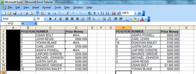
– Or, alternatively, as above, the format of the data in your reference columns is ‘text’. You can fix this in one of two ways:
– i) the EASY way is to insert a column after your first reference column (so insert a column in between cells B and C, then type the following formula in cell C2:
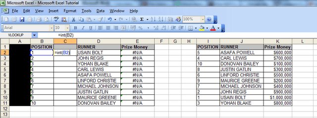
=int(B2) then press ‘Enter’ (see screenshot below). After pressing ‘Enter’ drag down the formula so that all the cells in column B are made into ‘integers’ in column C. Now highlight the numbers in column C, copy them, then highlight the cells in column B and click ‘paste Special values’. Now delete column C, and your vlookup will work, like magic!!
– ii) the OTHER way is to change the format of each cell in col B to ‘general’, click ok, then press F2, then press Enter. (NB You must carry out those steps in exactly that order, otherwise they won’t work! Make sure after changing the format of the cell to ‘general’ and clicking ok, that you press F2 BEFORE pressing enter). However, with this method, you would have to do one cell at a time, which is time-consuming. I’m here to save you time!
5) vlookup #N/A error because wrong ‘lookup value’ is used in the formula
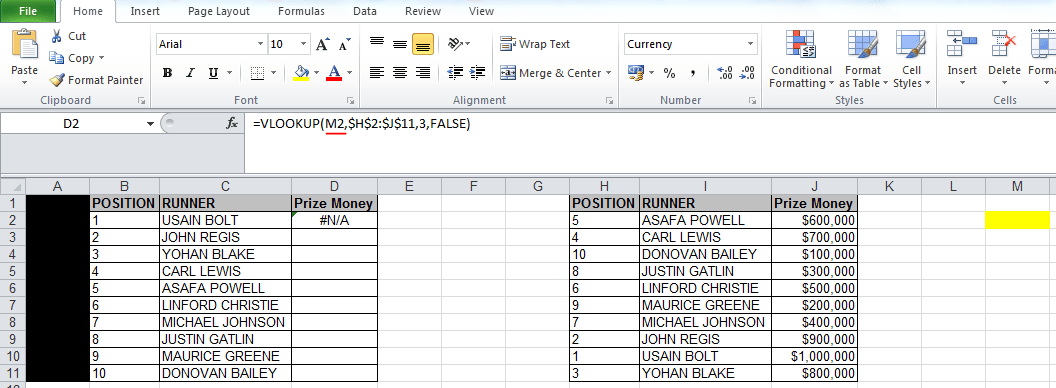
In the formula in the screenshot below, you can see the formula
=VLOOKUP(M2,H:J,3,FALSE)
It has 4 different arguments which combined together create a vlookup:
=vlookup(lookup_value, table_array, col_index_num, [range_lookup])
However, the thing that’s wrong in this formula is the ‘lookup value’ – it is M2, when it should be B2. M2 is far away from both tables – see the cell highlighted in yellow. So simply changing M2 to B2 in this case will make the formula work ie the error is the first part of the formula, also known as the ‘lookup value’
6) vlookup #REF! error
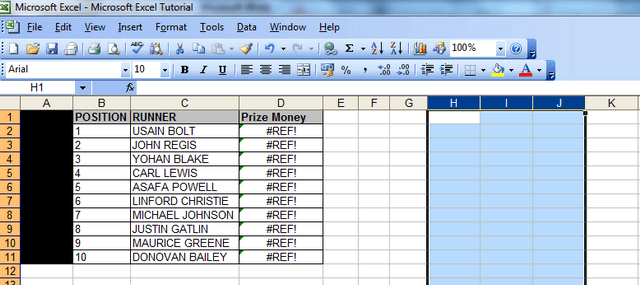
This will happen if the file, spreadsheet or table array that you were looking up data from has been deleted. An example of this is below, where I have deleted columns H to J and the vlookup described in the example above is returning the #REF! error.
7) vlookup #REF error because table array is incorrect
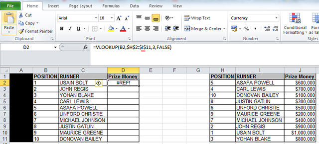
In the screenshot below, the table array consists of 2 columns instead of 3 ie H to I instead of H to J.
The formula is trying to extract the “Prize Money” values in column J, so the formula needs to go up to column J to capture the information in that column!
Otherwise, the formula won’t work! Changing the letter I to J in this case will make the formula work.
8) vlookup not working for some cells/vlookup not working sometimes
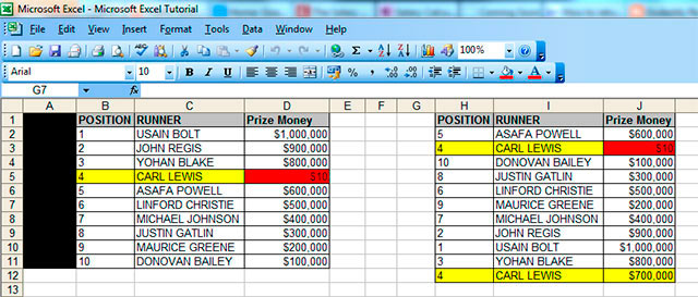
– if this happens, it is usually because your unique value is listed more than once in your reference table. And it would also have different values assigned to it. The screenshot below illustrates what I mean.
– The number “4” appears twice in column H in the table on the right hand side, so the vlookup formula returns the first value assigned to the number “4” in that table, which happens to be $10 (highlighted in red) in column J. If that row was deleted, then the vlookup would return the next value that it found assigned to the number “4” in that table, which would be $700,000 (highlighted in yellow at the bottom). In this example, $10 “Prize Money” is an unlikely amount for any athlete to get paid, as you can see all the other values are much higher, so the vlookup is returning the wrong result. To fix this, you would need to delete any duplicates that are irrelevant in your reference table.
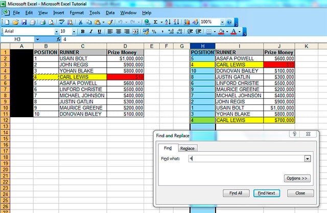
– to find out if a value is a duplicate in a spreadsheet that you’re working on, copy your unique value from your first table, in this case “4” in column B on the left hand side, go to your reference table or the other data that you are looking up (table on the right hand side above) and press ctrl+f then paste your unique value in the field that comes up shown below. Click on “Find Next” and Excel will move to each row where it can find the number “4” whenever you click “Find Next”. If it appears in the table more than once, then you’re likely to find that your vlookup is returning the wrong data.
9) vlookup not working – just showing formula.
If your vlookup isn’t working, and is returning the formula like this (see cell D2)
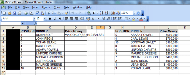
then you need to
– left click into the cell where the formula isn’t working
– right click and choose ‘format cells’
– you will notice that the current format is ‘text’
– change this to ‘general’
– click ok
– then press F2
– then press ENTER. You need to ensure you press F2 before pressing enter, otherwise this won’t work.
– after you’ve done that, the problem will be fixed and you can drag the formula down to other cells in the column, if necessary.
10) sum of sales data not working because some vlookups are returning N/As:
You may have experienced a problem at work where you are analysing data, and you have a spreadsheet with vlookups and a ‘sum function/total value formula’ at the bottom of each column with the vlookups. However, your sum function may be returning the word “N/A” instead of a total value or an actual figure.
You can fix this by changing your vlookups so that if they don’t find a value, they return a “0” instead of an “N/A”. The sum function will usually not work if there are “N/As” in the column concerned.
I have added in an extra row here (with Donald Trump as runner) to illustrate the above problem.
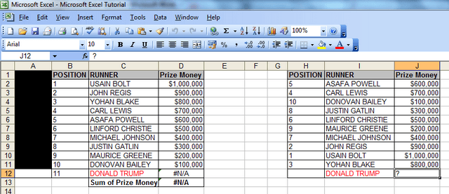
To fix this, you need to add an IF statement to your vlookup. Let’s take the vlookup formula in cell D11 which currently looks like this: =VLOOKUP(B12,H:J,3,FALSE)
If you add the following text, the formula will return a “0” instead of an “NA”, and this will allow the sum function (=SUM(D2:D12)) in cell D13 to work. So just add these bits (I would suggest putting an apostrophe in front and writing this formula in a separate cell first):
i) ‘=IF(ISERROR
ii) copy and paste your original vlookup straight after the above ie (VLOOKUP(A2,I:M,5,FALSE)
iii) add the following ),0,
iv) then paste the original vlookup again (VLOOKUP(A2,I:M,5,FALSE) and add two brackets )) at the end to finish the formula (if you then take out the apostrophe and paste the formula into cell D11, the vlookup will return the value “0” and your sum function//totals formula will work.
v) the revised formula will look like this: =IF(ISERROR(VLOOKUP(A2,I:M,5,FALSE)),0,(VLOOKUP(A2,I:M,5,FALSE)))
The above formula basically says “if there is an error with the vlookup, return the number “0”, and if there isn’t an error, then return the value that the vlookup is looking for.
NEW UPDATE!!!
There is an alternative and SHORTER version of the above formula which can be used in Excel 2007 onwards – thanks to one of our visitors (Joe).
It uses the IFERROR function.
We’d simply just take the original function that we have ie (VLOOKUP(A2,I:M,5,FALSE) and add the word “=IFERROR” at the beginning and “,0)” at the end so it would look like this:
=IFERROR(VLOOKUP(A2,I:M,5,FALSE),0)
Less common but very annoying vlookup problems (when you don’t know the solution)
11) #NAME error – because of incomplete ‘argument’ in the formula
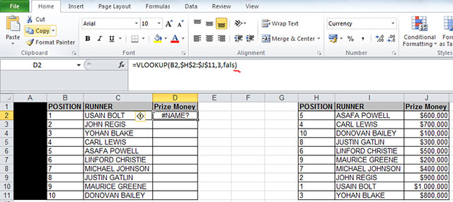
In the example above, everything in the formula is fine except for the last word, which is “fals” instead of “false” with an “e” at the end.
So if you’re using words in formulas, it’s important to spell them correctly, otherwise you’ll get an #N/A error.
12) vlookup not working when using a 2007 (or 2010) Excel file and you’re looking up data from an Excel 2003 file (or vice versa).
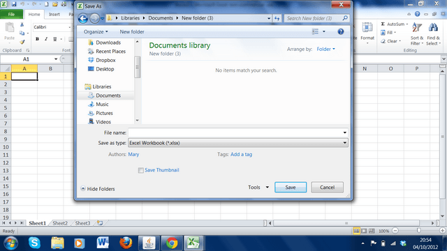
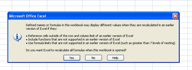
– in the Excel 2007 or 2010 file (s) [NOT 2003], click on ‘file’ then ‘save as’ then in the ‘save as type’ drop down menu at the bottom of the ‘save as’ pop up window, change file type from ‘Excel workbook (*.xlsx)’ – see screenshot below – to ‘Excel 97-2003 Workbook (.xls)’. You will then get the error message shown below in the second screenshot below, at which point, you click ‘yes’. Your vlookup between the files will now work!
13) vlookup invalid error / vlookup invalid reference error
– If you’re working with large spreadsheets, ie those that have over 65,000 rows, you’re likely to come across the “vlookup invalid error” – the “invalid” message appears next to the table array field (see screenshot below). If you complete the vlookup anyway, you’ll then get another error message (see second screenshot below) which says “Invalid reference. This file version can only have formulas that reference cells within a worksheet size of 256 columns (column IW or higher) or 65,000 rows.
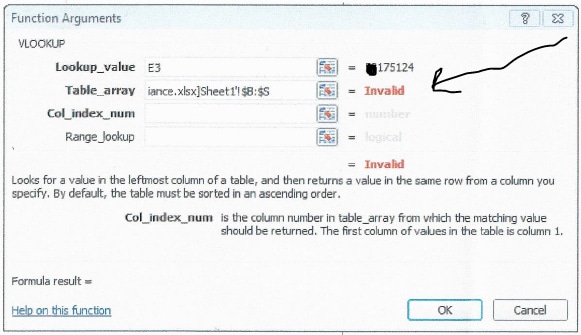

The solution here is two-fold:
i) Ensure that if your table array has more than 65,000 rows, you put anything between rows 65,0001 to 130,000 in a separate sheet, then put anything from rows 130,001 to 195,000 in a separate sheet, and so on, in increments of 65,000, because that’s the maximum number of rows the vlookup function will look it.
ii) Ensure that rather than highlighting the columns (for your table array), you highlight the specific range of cells you’re looking up and “fix them” by pressing F4 – in the example on this site, the specific range for the table array would be cells H2 to J11 – you can see this by either downloading the spreadsheet – available at the top of the site; or simply looking at the screenshot in problem number 5 above.
Hope that’s solved all your problems! Have a nice day!
We ask that you take a moment to read our Terms and Conditions and Privacy Policies.
I’m using my spreadsheet…..I cannot use the sum function, add results from vlookup cells….if I sum them together the results comes back as #VALUE!
what can I do…..
Hi Gil
What type of results are you trying to add up? Can you send a file with 2 examples?
If you’re trying to sum up two cells, the #VALUE error only comes up if the two sets of data are incompatible eg if you tried to add the word “Grey” to the number “1”, you’d get a #VALUE error, because you can’t add numbers and words together in Excel.
When using VLOOKUP, the first cell works, but when dragged down from the first cell, all cells return the same value as the first cell even though the formula in each cell is correct..
The only way to rectify is double click each cell and press return, however this is very time consuming
Any ideas please?
Hi
The calculation of your cells are most likely set to manual rather than automatic.
In Excel 2007 or later, click the Office button / Excel options / Formulas then select “automatic”.
Let me know if that doesn’t fix your problem.
Hi, it has been so long since I play with VLookup and now facing the same old problem. I think I put the formula correctly but still get #N/A result. I am using my own data for office management documents. Please help…
Hi Azza
Apologies for the delay in responding.
I have been unwell with the flu. If the info in your spreadsheet is not confidential, please send it through. The only other reason you would get an #N/A error is if your formula has not been put in correctly. I will be posting a new #N/A error on the site soon from another user who had an incorrect formula.
Hi Analyst,
Kindly share me your email address so that I can forward you the data. Million thanks.
Hi,
Already sent you the data. Hope to hear from you real soon! 😀
I’ve e-mailed you back directly.
Hi, hope you well. I urgently need help, I’m working on a workbook and my vlookup keep on showing #N/A, I’ve checked all the options and still don’t know where I’m going wrong. Please help?? Can I please e-mail you the workbook to check and inform me where I’m going wrong to prevent this from happening.
Thank you
Hi Chica
Yes, you certainly can, assuming that it doesn’t have any confidential info.
Thank you, please forward your e-mail address?
Hi
Just seen these, but we’ve already communicated via e-mail.
THANK YOU. I am new to VLOOKUP and could not figure out what I was doing wrong! I had problem #1.
You’re welcome.
thank you, my formula finally worked it was the invisible dashs that was stopping it from working.So happy now.
Great – glad your problem is resolved now.
Hello,
When i use vlookup (using excel 2013) it has returned with the same value as of top most cell in all the cells can u please help on this.
Hi
I’d need to know two things:
i) the formula you’re using, to check if it’s correct and
ii) if there are any duplicates in the file that you’re looking up.
If you send the answers to these questions, then I can assist further.
I have a vlookup function that is returning 0 for a value. I made sure all my lookup values were general, double checked my table array to make sure the lookup value did not appear multiple times. I tested using other values that showed up in the array above and below, above worked but below did not. Is there a limit of how vlookups you are allowed to do in a table. I have 8, the first 7 work perfectly but number 8 returns a zero every time. Thank you.
Hi Kevin
Can you send sample data, assuming it’s not confidential? I’d need to see the formula you’ve used, as without seeing the file you’re describing or any of the formulas in it, I can’t tell why it’s working for some cells but not others. It’s bit like a car mechanic trying to fix a problem under the bonnet of a car without opening it.
Hi,
I’m trying to do a Vlookup and continue getting no result, where nothing populates the cell other than the formula. I’ve reformated the cell to ‘General’, but still continues to show only the formula? Any suggestions?
Thank you
Hi Todd
Solution number 7 that I’ve described above has ALWAYS worked for this problem. However, you need to ensure you press F2 after changing the cell to ‘General’ then press the ENTER key – apologies, I’d left that last bit off, but have included it now, as it’s something I did automatically, and other visitors had posted comments on this page saying that the solution worked for them.
Let me know if you still need help.
I am doing a simple Vlookup and it is returning N/A. I need to return 0-25 = LOW and so on. Formula is =VLOOKUP(C7,B19:C22,2,) there are no spaces, and the tables are formatted as numbers.
Please help!!
Hi Vickie
Without seeing your file, I can’t tell exactly what’s gone wrong but I can tell you that you always need to put the word “FALSE” at the end of a vlookup formula.
So if the rest of your formula is correct, then the completed version should look like this: =VLOOKUP(C7,B19:C22,2,FALSE)
Try that and let me know if you still get the error.
For your #8 solution instead of using =IF(ISERROR(VLOOKUP(A2,I:M,5,FALSE)),0,(VLOOKUP(A2,I:M,5,FALSE))). It might be easier to use the IFERROR function because the formula is much shorter and therefore there are less opportunities to make a mistake. In the case of your example, it would be: =IFERROR(VLOOKUP(A2,I:M,5,FALSE),0) to produce the same results.
Hi Joe
Thanks for the suggestion – yes – that’s true, however, the function you’ve used wouldn’t work in Excel 2003 or any other versions before Excel 2007.
I wrote the content for the site a while ago, when many people were still using Excel 2003. The solution I’ve given works in all versions of Excel, but I’ll add your yours to the list, along with a number of other solutions that I’ve resolved for readers privately.
I just need to get the time to add all the new content.
Thanks again.
When I copy the vlookup formula and paste it below, the same value is returned. Now, if I go to the next cell and open the formula and hit ok, the correct value is returned. Can you assist?
Yes – I’ve emailed you directly.
Can you please share? This is the exact problem I’m having. Thanks in advance.
Hi,
I’m working on a project and I can’t get the F4 function to work to lock in the view. I have to multiply the formula down the columns many times. Is there another way?
Hi Emery
Yes – two alternatives –
1) for the table array, you can either simply highlight the columns you need – as illustrated in Step 5 in the tutorial on this page: https://howtovlookupinexcel.com/ or
2) clear the table array field then rehighlight the range of cells and then press F4 BEFORE pressing anything else.
Let me know if you’ve got any further questions.
PS to add to my previous note.
In my left hand columns, the figures are correct, but, there are no dollar signs or commas. How would I correct this, or do to change this in another test ?
Hi Ray
Glad I could help. The dollar signs and commas should appear, but if they don’t, then you can just highlight the cells concerned, right click, choose “format cells” then click on “currency” and select the number of decimal points that you want to appear. Let me know if that’s not clear.
I am having issues with VLOOKUP. There are several EIN# and LOID. It matches the values of the lookup but sometimes it will do say 10 out of 20 and the rest 10 are N/A.
Have spent hours and cannot figure it out. Did you the steops you have mentioned.Please help!
Hi Purnima
I suspect that there may be an error with the way your formula is written. If the file doesn’t have any confidential information, please send it to the email address that you get this response from and I’ll have a look for you.
Hi! Is it possible to use vlookup if the value you are looking up are words?
I am trying to populate a column with employee names. and the only data I have to pull from are the store name the employee is associated with.
For instance:
On Table is where I am trying to fill employee names:
Store Name Rep Name
ABC
On Table two, i am pulling the info. I have:
Store Name Rep Name
ABC Jane Doe
The store name are spelled the exact same way on both sheets and I continue to get an N/A when trying to get the rep name to populate!
Desperate!
One more question, if you don’t mind. When you use =If(iserror), etc, does that work no matter what comes back n/a, invalid, #ref, etc?
What happens if you write =if(isna) etc.?
I’ve written back to you directly.
Thanks for these great tutorials.
There’s one concept here I don’t understand. Why do we need to put the dollar signs to lock in a specific range of cells, but we don’t need to lock in if we just choose a range of columns?
What would happen if I chose a5:h8, without locking it in?
In general, I’m trying to understand the concept so I’ll have an idea of when I should lock in a range, and when I should leave it open.
Thanks a lot, this solved my problem perfectly (#7)!
Hi Vlookup Analyst,
I’ve been using Vlookup successfully in other worksheets in my file. But when trying to use it again, using this sheet, I constantly received wrong answers (the first 3 lines are OK, but then the results look ‘random’, and are actually returned from wrong lines).
No matter what I did, I could not find a solution to this behavior.
I reduced the wrong behavior to doing Vlookup on a simple table that only needs to return the same lookup-value, and still the answer is wrong.
I’ll be glad to send the file to you.
Thanks a lot,
Ophir
Hi Ophir
If the info isn’t confidential, please send it to the email address that you get this response from and I’ll fix the problem for you.
I am having the same problem as #10. I am trying to locate items on one list, but not on another.
If the info you’re analysing isn’t confidential, then send it through to the email address you get this response from and I’ll have a look.
I have tried all of these solutions and am still getting #N/A in multiple cells, although I’ve replaced it with an empty syntax with IFERROR. Other cells in the same column return with the information I need and the table is simply the columns instead of a specific range.
I’ve triple checked extra spaces and number values. Can you possibly take a look and see what I am doing wrong?
Hi Danielle
Yes, I’m happy to take a look. I imagine that it could be to do with the range you may have selected. If the info isn’t confidential, please send it to the email address that you get this response from and I’ll fix the problem for you.
For reasons unknown, my data just starts displaying #N/A at a certain number.
Tried a number of solutions above, nothing seems to fix it :/
Help!?
Hi Jess
Are you using a file from this site or your own? If your using your own file and it doesn’t contain confidential data, send it to the email address that you get this reply from and I can have a look.
Analyst.
Hi there,
Thank you for the great tutorial.
I am having issues with one file. I get the wrong number pulled when I highlight the columns but it works fine when I select the range of data in the table. Does anyone know why that is?
Thanks,
Caroline
Hi Caroline
Are you using a file from this site or your own? If your file doesn’t contain confidential data, send it and I can have a look.
There is also a setting (for 2010, it’s under Excel Options / Formulas) that allows the user to either manually or automatically calculate formulas.
Somehow, this got set to manual for me, which caused me to lose two hours debugging for nothing!
Hopefully this comment will help others…
Good Lord! I’ve lost almost a full day of work because I couldn’t get ANY formulas to work. This tip was a life saver! THANK YOU!
You’re welcome.
I continue to receive the #N/A error and have checked ALL the recommendations you posted to no avail. These are large files. Really could use some help.
If you send me a sample of the file, providing it doesn’t have confidential data, I can investigate the issue for you. I’d be very surprised if it isn’t covered in the list above, but I’d need to see your file to see for myself. Otherwise, it’d be like a car mechanic trying to check what’s wrong with a car without seeing it.
Totally understand diagnosing without looking. Please send me your e-mail and I will forward a small portion of the file.
Thanks in advance,
Nancy
Lo and behold, when you take your car to the mechanic, it no longer makes “that” noise.
A column was formatted as text but not visible. There was not a triangle in the corner, nor did it show in the formatting screen. Go figure, but all is working now.
Thanks for your help and I’ll be sure to refer to the site in the future.
Regards,
Nancy
Ha ha! Glad everything is working for you now. If it recurs, let me know.
Does the information have to be in a specific order? I have column A as acct #s and column B is the name. I need to get the acct#. I can’t get vlookup to work unless I change the acct # to column B.
Yes – vlookups can only obtain data from the RIGHT. You can do a reverse vlookup – I’m writing content for it and will let you know when it’s ready. Alternatively, if you send me your file, providing it doesn’t have confidential data, I can write the formula for you.
Hi
I am using Vlookup to return values from a table in a seperate workbook. I get the #REF error unless the workbook that contains the table is open.
If I go to Data -> Edit links and choose “update values” it still doesn’t work but if I choose “open source”, then the lookups work fine.
Does it have something to do with the fact that the data is in a table ?
Hi Steve
I’ve never come across this kind of problem before, to be honest. The REF error usually occurs if the data in the sheet you’re looking up is missing (as described in problem no. 5 above). A REF error could also occur because of an error in the formula, but I’d have to see the file you’re working on to make a fully informed view. If the data isn’t confidential, you can send it to the email address that you get this update from. But on the other hand, if your problem is solved and you’re happy then you can leave it as it is.
Very helpful page. One suggested addition – nonbreaking spaces. Ran into a VLOOKUP problem today, tried everything (including all your suggestions).
Turned out that certain cells contained nonbreaking spaces instead of the regular kind. Ctrl-H sorted it for me.
Thanks a lot for the valuable help. My vlookup problem got solved immediately.
You’re most welcome.
I use the reference from the first sheet but when I go to the table array and I want to select the reference from the second sheet it does not allow me, it just highlights the cells but not giving me the option to select the cell number?
Are you doing it using the spreadsheet I’ve provided on this site or are you using your own spreadsheet? If you’re using your own spreadsheet that issue is likely to occur because of the formatting in the spreadsheet. Also, which method are you using – highlighting the columns (like in the tutorial) or “locking the table array”, which is the alternative method described in step 5 on this page: https://howtovlookupinexcel.com/ ?
hi,
i am unable to extract birthday in this month form a employee list by using vlookup can you show me how to write vllokup with example. and send to me to my in box.
regards
n.k.prasd
I’d need to see your file.
Hello,
I try to put the Vlookup formula on a file which has been downloaded from a database. result is always N/A#. The data are alphanumeric. I already tried to reformat from General to Text, used the TRIM, CLEAN, INT functions, but nothing helps.
What can I do more?
If the data isn’t confidential, send me a copy of the file and I’ll have a look. Otherwise, I’d need at least a dummy version of the file to see what’s wrong – I’d need to verify that you’ve tried all 4 #N/A errors listed on this site.
I am having a strange issue today. I am doing a vlookup on an email address from 1 file to another and I am getting all #N/A results. I knew there was at least 1 match and when I go to that cell and click on the fx button in the formula bar and click OK then my match comes up. If I drag the formula from the cell above down again I get #N/A. I checked and the formula does not change from dragging it down to clicking the formula button and clicking OK. Any idea why this is happening? I tried saving my files in both 2010 and 97-2003. I can’t manually go to every cell and click the formula icon and OK to get accurate results.
I figured out the issue. File–>Excel Options–>Formulas tab. Somehow my setting was changed from Automatic to Manual. All fixed!
Hi Bridget
Apologies for the delay in responding. Yes the “manual” / “automatic” issue is a fairly common problem, but very easy to fix, as you’ve gathered.
I have a very simple vlookup that is retrieving the wrong data! I am looking up a cell from sheet2, on an table in sheet1 and it should be grabbing the data from the next column to the right, but it is pulling some random numbers instead. Any ideas?
Hi Tyrone
If it’s pulling the wrong data, then the formula hasn’t been written correctly. I’ve got a strong feeling that the problem is what I’ve described in problem number 3 on this page: https://howtovlookupinexcel.com/10-common-problems-with-vlookups. Please refer to that. If it still doesn’t solve your problem, and your file doesn’t have any confidential information, send it through, and I’ll have a look.
I’m having trouble getting a VLOOKUP function to work. It yields an “#N/A” result in each cell the formula is used. The data for the table_array is contained in a separate Worksheet within the spreadsheet. I just did a successful VLOOKUP in a separate spreadsheet using the same method but cannot get this one to work. As best I can tell, I’ve tried all of the above solutions and none have corrected the issue.
Hi Michael
If the information you’re working on isn’t confidential, then you can e-mail me at the address that you get this response from. Otherwise, I’d need to see a “dummy” version of the file (perhaps the first 5 lines of the sheets you’re referring to) to verify that you’ve gone through the 4 different #N/A errors described above and to see if there could be any other reason. Without seeing the file you’re working on and hence not knowing the format, etc I can only guess.
I’d me more than happy to send a copy of the information, but I didn’t receive an email because I neglected to check the box. I’ve checked it this time. Feel free to send me a message with the email address. Thank you!
Hi Michael
I’ve e-mailed you back.
Let me know if you don’t get the e-mail.
Done. I’ve e-mailed you directly.
Getting Vlookup errors the same as Number 1 on here.
Changed the entire column to ‘Number’ by highlighting the column and changing in toolbar. When I click on the cell with the green triangle in the left corner, it shows that it is in number format, however, the exlamation point still says ‘saved as text, change to number’. When I change the cell to number this way, even though it says it is already number, it will pull the information from the original workbook.
And not all cells have this error, which is why it’s more confusing! Roughly 75% of the values are pulled, only about 25% have this error.
Data in the original workbook shows as ‘number’ format also.
I have about 20,000 rows though, so I can’t click the exlamation point for all of them!
??
Note: My values contain numbers, letters, hyphens, slashes, and aterisks. (They are virtually SKU’s)
Ex:
400000RC3-215-0000
BCKFL16WOH
247/61293
Hi Lauren
If you have values that contain characters that are not numbers eg “400000RC3-215-0000” or “BCKFL16WOH” then using the “convert to number” solution won’t work as some of the characters in the cell are text based ie letters.
The “convert to number” solution only applies to products with numbers only as their unique ID, which I believe explains why some cells in your spreadsheet are not getting the error message. Is there another unique ID that you can use for the products? If so, I’d suggest using an alternative that does not contain a mixture of numbers and letters, but just numbers only. It looks like you may be using UPC codes and other IDs but I’d suggest using the SKU numbers only. Hope that helps. Let me know if it doesn’t.
I did “text to columns” for the SKU column, and for the SKU columns of all the workbooks I was pulling from and it fixed the error. I don’t know what text to columns does really, but it somehow fixed the problem!
Ok, glad you resolved the problem. Without seeing your spreadsheet, I could only guess what the problem was, and as you can see from the examples I’ve provided, there can be several different reasons why the function may not be working. From what you’ve described, it sounds like when you downloaded the data, it was all in one column, rather than several. This can be a default setting with some software systems. Text to columns basically splits the data in to separate columns – a simple example is explained here: http://office.microsoft.com/en-gb/excel-help/split-names-by-using-the-convert-text-to-columns-wizard-HA010102340.aspx Let me know if you have any other questions.
That worked.. Change the formula format to ‘general’. Thanks!
No worries.
Got a #ReF! error when I tried to copy paste the data I earlier did a Vlookup on. Cant tell why, because the data is not deleted and it is very much present. So i just went to Home –>cells–>format–>cell lock. then i got then the appearance of these cells changed i.e. there was green mark on them and then, i could copy paste these cells to the other sheets. Just something i tried. I just want to make sure if this wont lead to any Problem in the future with my data.
Hi
I’d need to see the spreadsheet you were working on. If you can re-create the problem with some example data, then drop me an email, I can have a look.
VERY helpful for someone who has recently begun using Vlookup! Thank you!
Thank you very much for these great tutorials. I really appreciate your effort.
Good luck.
Thanks for the compliment.
Thank you very much. I am enrolled in a cert4 Bookkeeping course. I have never used Vlookup before. It is in my new assignment and it looked just too hard to take in. But thanks to you I can now understand it, after completing the Runners & Prize Money scenario successfully. I did have a problem with #REF, but again with your help solved that too.You made it so easy to follow.
I guess that the tutors can do it with their eyes closed and forget how difficult things can be for their students at times to follow the first time round.
Thanks heaps again!!!