We’ve covered more vlookup problems than any other site on the internet
vlookup #N/A error? There are FIVE different #N/A errors and two different #REF errors explained below, as well as others such as the “Invalid reference” error. If you experience a different #N/A or #REF error to the ones listed below, then tell us. We’ve discovered new errors as a result of engaging with site visitors. But please check the solutions listed below first!
This page assumes you already know how to do a vlookup – if you don’t know how to, click here for the link to the 2007/2010/2013/2016 tutorial or here for the 2003 tutorial. The file with the data for the tutorials is here – once you’ve done a vlookup in column D as explained in the tutorials, you can replicate the problems below, if you wish. You can also just review the list below to find the problem you are experiencing.
- vlookup number stored as text (#N/A error)
- vlookup trailing spaces error AKA “the invisible dash!” (another #N/A error)
- vlookup #N/A error (because wrong range of data is selected)
- vlookup #N/A error (because data is missing from table)
- vlookup #N/A error because wrong ‘lookup value’ is used in the formula
- vlookup #REF! error because data is missing
- vlookup #REF error because table array is incorrect
- vlookup working for some cells but not others
- vlookup not working – just showing formula.
- Sum of sales data not working because some vlookups are returning N/As
- #NAME error – because of incomplete ‘argument’ in the formula
- vlookup not working when using a 2007 (or 2010) Excel file and you’re looking up data from an Excel 2003 file (or vice versa).
- vlookup invalid error / vlookup invalid reference error
1) vlookup number stored as text (#N/A error)
This is a formatting error that is very easy to fix!
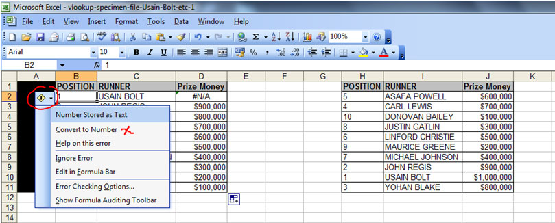
If you get an “N/A#” error and there is an exclamation mark next to the unique value used for your vlookup (see cell B2 in the screenshot below) then you simply have to click on the exclamation mark box the click on “Convert to Number.”
This will change the format of the cell from “Text” to “Number” and the vlookup should work. If it still doesn’t work, read on for other N/A errors covered on this page.
2) vlookup trailing spaces error AKA “the invisible dash!” (another #N/A error)
Some company reporting systems automatically generate reports where each unique value in the report has a trailing space at the end, which causes the vlookup to fail. This is the most difficult “N/A#” error to spot if you’ve never come across it before, as everything “appears” to be normal to the naked eye!
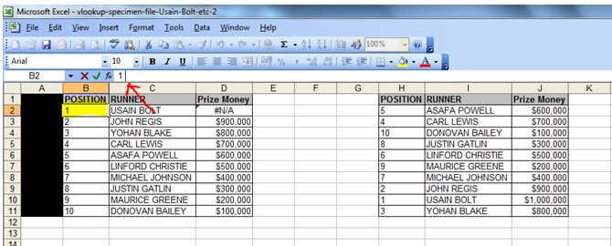
The unique values in the table below are in column B (the positions of the runners). I’ve highlighted cell B2, which has the runner in position 1 – in the toolbar, where the number “1” is shown ABOVE column C, there is a trailing space at the end (see red arrow) which caused the vlookup to fail and create an “N/A#” error in column D.
There are a number of solutions for this:
2a) the “Data – ‘Text to Columns’” solution.
Go to “Data” in the tool bar, then click on the “Data” tab (it’s in between the “Formulas” and “Review” tabs).

Now – and this is an important step – highlight the column where your lookup values are. In the main example on this site, the lookup values are in column B.
Then click on the “Text to Columns” icon in the tool bar.
![]()
Click “Next” in the window that pops up (make sure you leave “Delimited” as the file type).
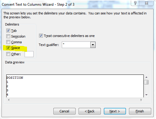
Click on the “Space” checkbox in the next window (see screenshot below). The “Treat consecutive delimiters as one” checkbox will automatically get ticket when you click on the “Space” checkbox. That is fine. Just click “Next” in the screenshot below. Then click on “Finish” and that’s it!
2b) take out the trailing space by clicking in the cell and pressing “backspace” at the end of the cell, to remove the blank space. However, this is time-consuming.
2c) click on the exclamation mark next to the cell then click “convert to number” – this is good, but it also a time-consuming solution.
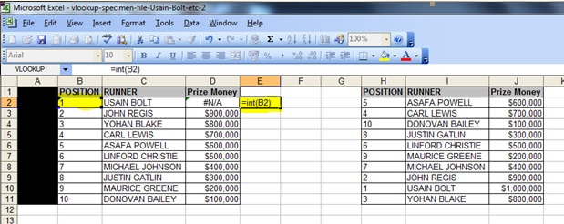
2d) Use the “=int” formula as demonstrated in the screenshot below – using a blank column, enter the formula “=int(” then cell number that you need to fix, in this case, cell B2, then close the brackets – the complete formula will look like this
=int(B2)
Now double-click the bottom right hand-corner of this cell so that the formula is dragged down and then copy the column from the cell where you first entered the”=int()” formula in this screenshot this is cell E2; and then click cell B2 (the cell that needs to be fixed) and then click file / paste special / values – this will convert all the cells in column B to “integers” and at the same time remove the trailing spaces. Voila!
3) vlookup #N/A error (because wrong range of data is selected)
Here’s a problem from someone who visited this site (and the solution, of course!)
Rather than use the method described, they’d started by typing “=vlookup….” and had selected an incorrect range of cells to look at.
They said they had doubts about the vlookup function and didn’t know how to use it properly.
They were getting an n/a error and didn’t know why! So I got them to send me the file available on this site to see what they’d done wrong. There were 5 N/A errors in their spreadsheet but I’ve left only one instance of the error in the file, to make it easier for you to understand why it happened.
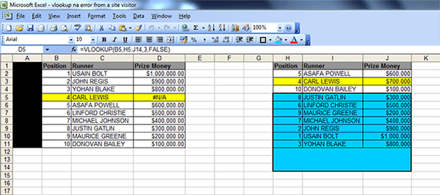
The cell with the N/A error is cell D5 (see screenshot above). It has an “N/A” instead of the value “$700,000”. You can clearly see that Carl Lewis is in position 4 in both tables (left and right); and if you look at the table on the right, the Prize Money assigned to him is $700,000.
Here’s a link to the file with the error, in case you want to see it in closer detail – LINK TO FILE
The non-technical language explanation for this is that their vlookup formula was looking for a result for Carl Lewis in the BLUE AREA, when the result for Carl Lewis is in the YELLOW AREA ie ABOVE the BLUE AREA. (The vlookup was referencing the runner in position 4 but I have used the runner’s name as it’s quicker and easier to understand).
The technical explanation is this: the formula they created in cell D5 was this =VLOOKUP(B5,H5:J14,3,FALSE) where:
B5 is the runner in position 4 in the first table – which is ok (this is the lookup_value)
H5:J14 is the BLUE AREA – which is NOT ok (this is the TABLE ARRAY)
3 is the column reference – which is ok (this is the column_index_number)
FALSE – which is ok (this is called the Range Lookup but it’s simply the last part of the formula to complete the argument and ensure an exact match is returned, and if not found, then an “N/A” is returned.
There are two solutions for this:
either use SOLUTION 1 which is =VLOOKUP(B5,H:J,3,FALSE)
OR use SOLUTION 2 which is: =VLOOKUP(B5,$H$2:$J$11,3,FALSE)
With SOLUTION 1, we are just changing the cell selection for the TABLE ARRAY from H5:J14 to H:J ie take out the numbers! Putting the wrong numbers in the TABLE ARRAY part of the formula will cause an “N/A” error. In this case their formula started at cell H5 (which is position 8) but it is BELOW the area where the result they’re looking for (position 4) which is in the YELLOW AREA.
With SOLUTION 2, we are fixing the range of data from which the formula will search for a result. However, we cover all the “positions”, “runners” and “prize money” in the range. The visitor’s range was missing the $ signs and the cells H2 to J4.
So you can either highlight columns H to J in their entirety, as explained in the tutorials (see step 5 here: https://howtovlookupinexcel.com/) OR – highlight the range of cells of the data you’re referencing.
4) vlookup #N/A error (because data is missing from table)
– this will happen either because the data you are looking up doesn’t exist (see table below where the numbers 1, 3 and 5 are not in the second table. You’ll notice that the ‘prize money for the runners in position 1, 3 and 5 in the first table is “N/A” instead of the actual value), so the formula returns an “N/A” instead of the result that you’re looking for.
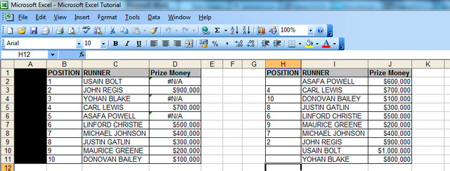
– Or, alternatively, as above, the format of the data in your reference columns is ‘text’. You can fix this in one of two ways:
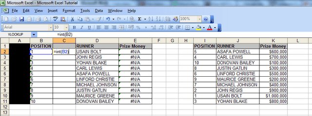
– i) the EASY way is to insert a column after your first reference column (so insert a column in between cells B and C, then type the following formula in cell C2:
=int(B2) then press ‘Enter’ (see screenshot below). After pressing ‘Enter’ drag down the formula so that all the cells in column B are made into ‘integers’ in column C. Now highlight the numbers in column C, copy them, then highlight the cells in column B and click ‘paste Special values’. Now delete column C, and your vlookup will work, like magic!!
– ii) the OTHER way is to change the format of each cell in col B to ‘general’, click ok, then press F2, then press Enter. (NB You must carry out those steps in exactly that order, otherwise they won’t work! Make sure after changing the format of the cell to ‘general’ and clicking ok, that you press F2 BEFORE pressing enter). However, with this method, you would have to do one cell at a time, which is time-consuming. I’m here to save you time!
5) vlookup #N/A error because wrong ‘lookup value’ is used in the formula
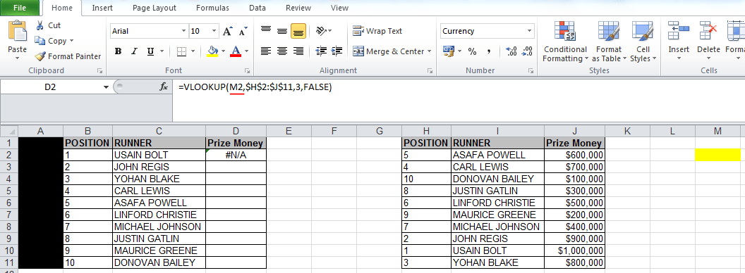
In the formula in the screenshot below, you can see the formula
=VLOOKUP(M2,H:J,3,FALSE)
It has 4 different arguments which combined together create a vlookup:
=vlookup(lookup_value, table_array, col_index_num, [range_lookup])
However, the thing that’s wrong in this formula is the ‘lookup value’ – it is M2, when it should be B2. M2 is far away from both tables – see the cell highlighted in yellow. So simply changing M2 to B2 in this case will make the formula work ie the error is the first part of the formula, also known as the ‘lookup value’
6) vlookup #REF! error
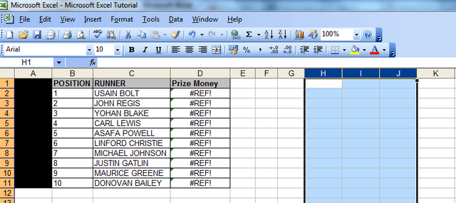
This will happen if the file, spreadsheet or table array that you were looking up data from has been deleted. An example of this is below, where I have deleted columns H to J and the vlookup described in the example above is returning the #REF! error.
7) vlookup #REF error because table array is incorrect
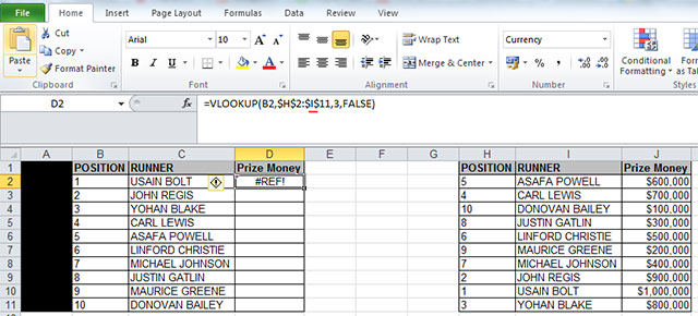
In the screenshot below, the table array consists of 2 columns instead of 3 ie H to I instead of H to J.
The formula is trying to extract the “Prize Money” values in column J, so the formula needs to go up to column J to capture the information in that column!
Otherwise, the formula won’t work! Changing the letter I to J in this case will make the formula work.
8) vlookup not working for some cells/vlookup not working sometimes
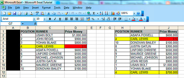
– if this happens, it is usually because your unique value is listed more than once in your reference table. And it would also have different values assigned to it. The screenshot below illustrates what I mean.
– The number “4” appears twice in column H in the table on the right hand side, so the vlookup formula returns the first value assigned to the number “4” in that table, which happens to be $10 (highlighted in red) in column J. If that row was deleted, then the vlookup would return the next value that it found assigned to the number “4” in that table, which would be $700,000 (highlighted in yellow at the bottom). In this example, $10 “Prize Money” is an unlikely amount for any athlete to get paid, as you can see all the other values are much higher, so the vlookup is returning the wrong result. To fix this, you would need to delete any duplicates that are irrelevant in your reference table.
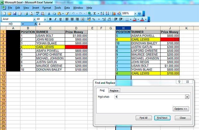
– to find out if a value is a duplicate in a spreadsheet that you’re working on, copy your unique value from your first table, in this case “4” in column B on the left hand side, go to your reference table or the other data that you are looking up (table on the right hand side above) and press ctrl+f then paste your unique value in the field that comes up shown below. Click on “Find Next” and Excel will move to each row where it can find the number “4” whenever you click “Find Next”. If it appears in the table more than once, then you’re likely to find that your vlookup is returning the wrong data.
9) vlookup not working – just showing formula.
If your vlookup isn’t working, and is returning the formula like this (see cell D2)
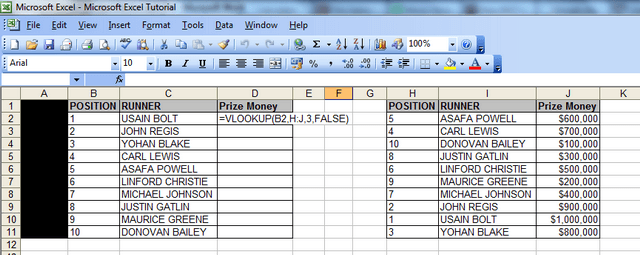
then you need to
– left click into the cell where the formula isn’t working
– right click and choose ‘format cells’
– you will notice that the current format is ‘text’
– change this to ‘general’
– click ok
– then press F2
– then press ENTER. You need to ensure you press F2 before pressing enter, otherwise this won’t work.
– after you’ve done that, the problem will be fixed and you can drag the formula down to other cells in the column, if necessary.
10) sum of sales data not working because some vlookups are returning N/As:
You may have experienced a problem at work where you are analysing data, and you have a spreadsheet with vlookups and a ‘sum function/total value formula’ at the bottom of each column with the vlookups. However, your sum function may be returning the word “N/A” instead of a total value or an actual figure.
You can fix this by changing your vlookups so that if they don’t find a value, they return a “0” instead of an “N/A”. The sum function will usually not work if there are “N/As” in the column concerned.
I have added in an extra row here (with Donald Trump as runner) to illustrate the above problem.
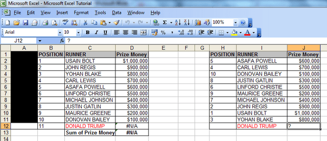
To fix this, you need to add an IF statement to your vlookup. Let’s take the vlookup formula in cell D11 which currently looks like this: =VLOOKUP(B12,H:J,3,FALSE)
If you add the following text, the formula will return a “0” instead of an “NA”, and this will allow the sum function (=SUM(D2:D12)) in cell D13 to work. So just add these bits (I would suggest putting an apostrophe in front and writing this formula in a separate cell first):
i) ‘=IF(ISERROR
ii) copy and paste your original vlookup straight after the above ie (VLOOKUP(A2,I:M,5,FALSE)
iii) add the following ),0,
iv) then paste the original vlookup again (VLOOKUP(A2,I:M,5,FALSE) and add two brackets )) at the end to finish the formula (if you then take out the apostrophe and paste the formula into cell D11, the vlookup will return the value “0” and your sum function//totals formula will work.
v) the revised formula will look like this: =IF(ISERROR(VLOOKUP(A2,I:M,5,FALSE)),0,(VLOOKUP(A2,I:M,5,FALSE)))
The above formula basically says “if there is an error with the vlookup, return the number “0”, and if there isn’t an error, then return the value that the vlookup is looking for.
NEW UPDATE!!!
There is an alternative and SHORTER version of the above formula which can be used in Excel 2007 onwards – thanks to one of our visitors (Joe).
It uses the IFERROR function.
We’d simply just take the original function that we have ie (VLOOKUP(A2,I:M,5,FALSE) and add the word “=IFERROR” at the beginning and “,0)” at the end so it would look like this:
=IFERROR(VLOOKUP(A2,I:M,5,FALSE),0)
Less common but very annoying vlookup problems (when you don’t know the solution)
11) #NAME error – because of incomplete ‘argument’ in the formula
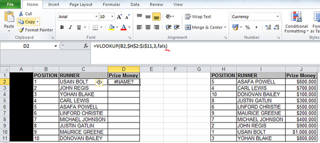
In the example above, everything in the formula is fine except for the last word, which is “fals” instead of “false” with an “e” at the end.
So if you’re using words in formulas, it’s important to spell them correctly, otherwise you’ll get an #N/A error.
12) vlookup not working when using a 2007 (or 2010) Excel file and you’re looking up data from an Excel 2003 file (or vice versa).
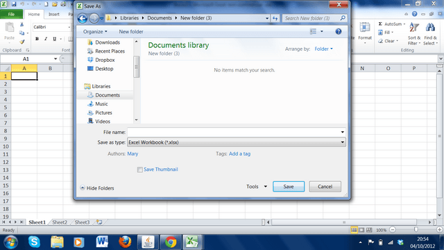
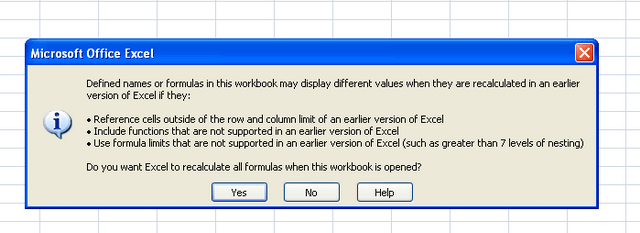
– in the Excel 2007 or 2010 file (s) [NOT 2003], click on ‘file’ then ‘save as’ then in the ‘save as type’ drop down menu at the bottom of the ‘save as’ pop up window, change file type from ‘Excel workbook (*.xlsx)’ – see screenshot below – to ‘Excel 97-2003 Workbook (.xls)’. You will then get the error message shown below in the second screenshot below, at which point, you click ‘yes’. Your vlookup between the files will now work!
13) vlookup invalid error / vlookup invalid reference error
– If you’re working with large spreadsheets, ie those that have over 65,000 rows, you’re likely to come across the “vlookup invalid error” – the “invalid” message appears next to the table array field (see screenshot below). If you complete the vlookup anyway, you’ll then get another error message (see second screenshot below) which says “Invalid reference. This file version can only have formulas that reference cells within a worksheet size of 256 columns (column IW or higher) or 65,000 rows.
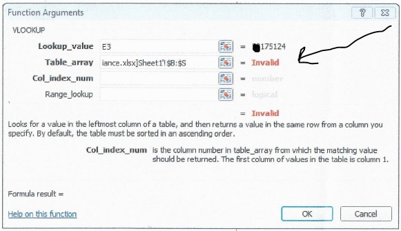

The solution here is two-fold:
i) Ensure that if your table array has more than 65,000 rows, you put anything between rows 65,0001 to 130,000 in a separate sheet, then put anything from rows 130,001 to 195,000 in a separate sheet, and so on, in increments of 65,000, because that’s the maximum number of rows the vlookup function will look it.
ii) Ensure that rather than highlighting the columns (for your table array), you highlight the specific range of cells you’re looking up and “fix them” by pressing F4 – in the example on this site, the specific range for the table array would be cells H2 to J11 – you can see this by either downloading the spreadsheet – available at the top of the site; or simply looking at the screenshot in problem number 5 above.
Hope that’s solved all your problems! Have a nice day!
We ask that you take a moment to read our Terms and Conditions and Privacy Policies.
I have a part # that includes “/” and, even when I copy and paste it from one sheet to the other (I have a main data vlkup spreadsheet that I use over and over) it won’t recognize the part #. Is it because of the “/”?
Hi Tracy
Apologies for the delay in responding.
If the “/” is in both sheets, then it shouldn’t be a problem.
However, you should check if there are any trailing spaces.
What’s the actual error that you get? And can you paste the part number from both sheets here?
Analyst
I was having the issue where sometimes the same vlookup worked and sometimes it didn’t.
Having checked the range was correct, I then fixed it in two ways:
1. make sure the left hand column is sorted in ascending order
2. select all the lookup data, copy to clipboard, clear the worksheet of all content, repaste as values only (no formatting)
Hope this helps your other readers.
Toby
Hi Toby
Thanks for your post.
You don’t have to sort your data in ascending order if your vlookup is done correctly.
But it’s good you found a way around the problem you had. I’ll post your comment on the site for others to see.
Analyst
I have a spreadsheet containing vlookups that when opened using Excel 2007 shows the values as intended. If I open the EXACT same spreadsheet using Excel 2010 or 2013 the values within the spreadsheet show up as #N/A. I am presuming that there is nothing wrong with the vlookups because they show just fine in one version of Excel but not the next. What could be the problem?
Hi Tim
Strange problem.
Can you copy and paste your formula here? With older versions of Excel, some functions don’t work eg “IFERROR” works before a formula from in Excel 2007 onwards, but not in previous versions of Excel, where you have to use “IF(ISERROR” instead.
Seeing what your formula looks like will help, if you can send it?
Analyst
I am using Excel 2016. I have a problem that is after using vlookup formula the result is #N/A but at the same time i gave Ctrl + S for save) the result had shown correctly. Like this after using right() the result was same in all columns at the same time i gave Ctrl + s the correct result had shown. How to correct this problem
Hi
It sounds like your calculations are set to manual rather than automatic.
Analyst
I encounted a PICNIC error that took me a while to figure out…
My spreadsheet somehow got changed to manual calculations. I was expecting some #NA’s but having autocalc turned off caused every result to be a #NA.
Hi Pat
Yes, if you opened a file from someone who had set their calculations to manual, the settings often transfer over to spreadsheets that you’re working on.
So it’s always worth checking the calcs.
Analyst
Is there any quick fix.
We have added many new rows to our sheet and now the vlookup is not working correctly.
How do i easily fix this as i am not a vlookup expert.
Hi Nicole
There’s two possible reasons:
i) the table array in your vlookup doesn’t included the new rows
ii) your vlookup is using a named range but the range of the data has changed because of the new rows that have been added.
If you download the files and watch the 5 min video we have on the site (https://howtovlookupinexcel.com/), you’ll become a vlookup expert in 5 minutes! Dozens of people have, as you’ll see from the comments on the site.
Let me know if you still have questions.
Analyst
Hello,
I have a question. I have a worksheet that has two sheets in it. Both sheets look at a 3rd one for the Vlookup. In some cases I don’t get a result from the formula. I only get N/A. But the same formula in an other line just over it works. The product that I’m looking for is in the 3rd sheet. Looked at it using copy/paste in the search box.
Now can it be because we have a long page of products? I will send you a copy of the file. It has no valueble information.
Thanks
Hi
I’ve responded to your e-mail.
Hi,
What was the answer to this question? Would be helpful as I’m having a similar problem.
I just lived through one more example of #NA that you may want to add to your list. Make sure the two spreadsheets are in the same folder location. I kept getting the #NA error until a friend asked me whether the spreadsheets were in the same folder on my computer. Of course they were not. I moved them into the same folder, reopened both spreadsheets and Voila! Formula worked.
Hi Mary
Thanks for your comment.
I’ve never had that problem before, as the location should not matter.
I vlookup information from different folders all the time.
But it’s good to share things, in case they’re useful for others.
Thanks
Sometimes we cant do Vlookup reason being one of the file will be shared. If we try to remove the share option or paste the info to a new excel – then the vlookup will work
I have apply vlookup formulla 100% ok , but here result is #name? why this is activities here?
Again Re applying this , but result is same. why?
Send me a copy of the file you used from the email address that you get this response from.
When the lookup cell (first column) contains text longer than 255 characters, vlookup returns #VALUE.
Hi Johann
I hadn’t personally come across that problem before, but it’s a good one to add!
Thanks
Analyst
Thanks! Your instructions about having an exact match, or VLOOKUP would not find the information in the lookup table, was very helpful.
I used people’s names to relate the spreadsheets, because there were no duplicates. Thanks to what you said, I realized my formula was not identifying Spanish surnames because the little accent over an “e” looked the same, but was actually different.
I cut and pasted the same name in both spreadsheets, so it is exactly the same, and it works!
Thanks
By the way, I would like to receive responses – but I don’t see the “notify me of follow-up comments via e-mail” box?
Hi Steven
Glad the instructions worked!
I’ll drop you an email about the follow-up comments.
Analyst
Hi,
Thank you so much. That solved the problem.
You are very helpful!
Hi, I have the same problem with Dominic White, the problem is the supposed to be B65 on my worksheet is a time duration which I got from subtracting the starting time from the completion time of a job, so when using int(B65) they’ll all set to 00:00.
As Dominic has explained, unless I type the value manually onto B65 the vlookup formula isn’t working.
Thank you.
Hi Lex
I’ve never personally come across this problem before.
But it sounds like a formatting issue.
If you send me a file with dummy data / data that is not confidential, I can investigate further.
Analyst
Hi, thank you for your response, where should I send my dummy data? I’ve checked my email and none from outside my colleagues. I’ve checked the formatting too, they seem fine, i don’t know what’s wrong with the data.
Hi
If you subscribed to follow up comments (next to the box where you post comments) then you’d receive an email from info@howtovlookupinexcel.com
If you send the dummy data there, I can have a look for you.
Analyst
I’ve sent the dummy data there. And I can’t find the subscribe button, seems like html error.
Hi
I’ve emailed you back.
I used the =TEXT(K2,”HH:MM”) formula to change the format of the time.
Can you please send me a screenshot of the html error that you get?
Thanks
Analyst
Hi!
I’m having the following issue with formula in my own datasheet.
=IF(VLOOKUP(J6,$C$243:$C247,1,0)=J6,”AAA”, if(VLOOKUP(J6,$C$250:$C$258,1,0)=J6,”BBB”, if(VLOOKUP(J6,$C$260:$C$287,1,0)=J6,”CCC”,0)))
I’m trying to put in a column(let it be “R”) one of the statements: AAA, BBB or CCC. In Column J I have countries. Underneath the table I’ve sorted these countries depending on VAT rate into 3 groups (C range). So instead of putting those AAA, BBB, CCC manually I wanted to create a formula. Instead in some cells I’m getting those three letters but in most cases (90%) I have #N/A. Why does it happen? Tried to take off 0 after the parameter 1, little bit better but still most of them have #N/A which says, e.g. Did not find value ‘UK’ in VLOOKUP evaluation.
Thank you!
Hi
It looks as though you just need a nested IF statement, rather than a vlookup with an IF statement in it. If the file doesn’t contain any confidential info and you have permission to share it, then send it through and I can help. If not, please don’t send it unless you have anonymised the data.
Hi.
Is there anyway to copy the formula across columns rather than down?
I am using a workbook with the months across the columns and the products in order down the sheet.
Thanks
Hi Janet
Yes, but you’d need to use an hlookup for that.
If you send a file with dummy data with three different columns in each workbook, I can do it for you.
Analyst
Hello,
Using my own spreadsheet. I created a VLOOKUP for one of the pages in a multi-page workbook and the formula works perfectly fine when I use it; the issue I am having is that I have four other people on my team, all running the same version of Excel, who use the workbook but VLOOKUP formula doesn’t work for 2 of them and does work for the other 2. Have you ever heard of an issue such as this or know any potential fixes I could try? I should mention that the workbook contains multiple other formulas, including other VLOOKUPs, all of which work perfectly fine for the 2 people for whom this particular VLOOKUP does not work.
Any suggestions you have are much appreciated!
Thanks,
Kelley
Hi Kelley
I’ve never heard of that issue, no.
But I’ll drop you an email with my thoughts on what may be happening.
Analyst
Hello. Thank you so much for this tutorial – it’s beyond helpful.
I am having one problem though…I was able to do the VLOOKUP using two of my own files and it worked perfectly for the first 2,630 entries, but every one after that shows as #N/A. The formula is exactly the same with the exception of the lookup value, which does correspond to the correct cell in all of the entries. All of the lookup values AND the results column are numbers and are formatted as “General.” (I can’t convert to numbers because they are zip codes and the ones that start with “0” are reduced to a smaller number (ie, “01001” is converted to “1001”).
Any thoughts on why this may be happening?
Thank you!
Hi Kathy
Thanks for your note.
Is there another unique ID that you can use to the do vlookup?
If not, I’d suggest that you insert a new column to the right of the column with the zip codes in both files, then convert the cells in those columns to numbers, then do your vlookups.
If you’ve got preceding zeros with the zip codes eg “01001” then there may be an apostrophe at the beginning of those codes to ensure the “0” remains in place, and this could cause the vlookup to fail.
Let me know how it goes.
Analyst
If the
Using my own spreadhseets.
“Table 1” has 15,000 records – It is a list of billing accounts and base billing rates. The data in this table is more or less fixed.
“Table 2” has 500 records which are billing adjustments for specific accounts. This table adds records over time.
I would like to insert the billing adjustment column from Table 2 to the end of Table 1 and subtract it from the base billing rate, resulting in a final bill amount.
Vlookup works successfully where there are matching accounts, but where there are not I am getting “N/A”, which I cannot use in my subtraction formula. I would like it to return a “0” instead. Is there a direct way to do this?
I attempted an IF function but have not been able to get a 0 to return successfully.
THANK YOU!!!
Hi Sean
Yes, there’s a really easy way of doing that. I’ve covered it in problem number 10 on this page: https://howtovlookupinexcel.com/10-common-problems-with-vlookups
However, if you’re stuck, send me your formula and I’ll edit it for you.
If you’re using Excel 2007 or later, all you’ll need to do is add “=IFERROR” before your formula then add “,0)” at the end of your formula.
If you’re using an earlier version of Excel, then I’ve described an alternative way that you can resolve that problem (also in problem 10).
Let me know how you get on.
Analyst
A ha! Perfect! Missed that in the discussion. Thanks so much, worked like a charm.
Ok, no problem.
Glad it helped you!
I have a file that for some reason is not returning a look up for a lookup of values I have that I am comparing between a file I have with banking details with a transaction file from the bank. Notice some of the differences you mention above but cannot see why some values that are sorted correctly do not return a value but rather a #N/A error. Can I send you a copy of an extract of the file to you? Tried using the Match function which likewise returns the #N/A error
Hi Paul
If you have a file with dummy / anonymised data, then yes, send it through and I can have a look.
Analyst
Hello, I saw this issue on a youtube comment and I was wondering if there was a remedy.
“…I have a table with over 20,000 items and some items might contain additional information that i dont always know, how can i create a formula that finds the first part of the item #, , most of my items are 8 digits long but then also have a space then other numbers,, example (900134142 120/60) ,or (900134142 24-60), is there a way or a special formula that will find these first numbers without having to know the last ones.?”
The solution provided by a person that DID NOT work for me was
“=VLOOKUP(VALUES(LEFT;3
What does this mean? Look for the first 3 digits starting from the left side of the whole number”
Also I was wondering, will this solution work with text? For example: I have first and last names in the same cell (1st column of Vlookup table), and they have values associated with them in a cell right next to them (second column of Vlookup table). But when I perform the vlookup function, the cell that is used as the “lookup_value” is just a first name. Can I only use first names to search?
Thanks in advance!
-Mitch
Hi Mitch
Apologies for the delay in responding.
Re your first question, I’d recommend just using the =left formula.
So if you have 8 characters (doesn’t matter if they’re numbers or text) in cell B2, for example, to get the first 5 characters, you’d just use =left(B2,5).
Re your second question, you can use names to do vlookups, but they’re less reliable than numbers, because the same name may have been spelt differently in the spreadsheets / columns that you’re working with eg John and Jon or Sam and Samy. Let me know if you have any other questions.
Analyst
My problem is similar to Solution number 8 above – only one of the vlookup values is just not being read properly = Team Leader. All other job roles are being read correctly. The vlookup function looks up the Team Leader’s YTD or Quarterly training target figure (in a table array) to check if this quarter’s value is below target and then marks it as 0% or 50%. There is another similar training target (makes up the rest of the 50% if both targets are achieved) which vlookups absolutely fine and is in the adjacent column of all relevant sheets.
Here are some strange anomolies which came up during troubleshooting. 1) If I change ‘Team Leader’ to random text, i.e. ‘Re’, ‘lead’, the vlookup sometimes works even if I don’t match it in the source table array. Shouldn’t it always be giving me ‘N/A’? Notably, it doesn’t work when i change it to just ‘Team’.
2) If I change the numeric value to 300 or above, the correct % comes up. Now, 300 is the number of the next row ‘Shift Manager’ target in the source table array.
I am 99% sure the formulas are correct as they are working in so many other columns. I have tried all possible solutions suggested from many excel sites and have extensively been using vlookup lately in which I have had to use many of the helpful solutions mentioned above – especially the Text to Columns one.
Hope you like a challenge and can help – my client is trying to finish his 3rd Quarter reports ASAP.
Thanks, Nals
Hi Nals
Re question 1), if you change the unique values you’re using to random text such as ‘Re’ or ‘lead’, the lookup formula would only work if your formula has the word ‘TRUE’ instead of ‘FALSE’ at the end, and if there was text with those characters in the table that you’re looking up i.e. ‘Re’ and ‘lead’ – if the formula has the word, true, then it will simply look for a related match rather than an exact one. What does your formula look like?
Re question 2), without seeing your file, and you should only send it if if you re-create a dummy version with different data, I’m not sure whether you are using words or numbers to do your vlookups – can you please clarify? You mentioned words in Q1 but you’ve mentioned numbers in Q2. This would make a difference. However, sending through sample dummy data would be the best thing, even if it’s just 3 rows of data.
Thank you for your response, very helpful. The formulas do not include the TRUE or FALSE at the end since they were nested within an ‘IF’ function. F4 & E4 refers to cells that have the job roles written in them and looks them up from the table array mentioned at the end.
=IF(F4<VLOOKUP(B4,YTD_targets,9),0,0.5)
=IF(E4<VLOOKUP(B4,YTD_targets,10),0,0.5)
cell B4 E4 F4
Team Leader 50647 1175262 205.5 4.0
Team Leader 50647 1175262 151.0 2.5 6.0
In reference to question 2, a sample of the table array is below. When i mentioned changing a value to '300' (the 'IF' part of the formula above) and it seemed to refer back to 'Shift Leader', I was referring to the below info.
YTD_targets – (lookup table):
col9 col10
Forklift Operator 7.0 0.0 0.0 0.4 0.0 8 32 32
Team Leader 7.0 0.0 0.0 0.3 0.4 0.0 60 24 40
Shift Manager 7.0 0.0 0.0 0.3 0.4 0.0 60 24 300
After adding 'FALSE' at the end, the correct information comes up, so that is great! I am still curious why it appears to work for all the other formulas without adding this, but not for Team Leader. Any ideas on this and do you recommend I go through all my vlookup formulas and add it in 'just in case' .
Thanks, Nals
Hi Nals
Glad the suggested solution worked for you.
vlookups should always have the word “FALSE” at the end. Some people put the word “TRUE” or the number “0” and others just leave that part blank. But I’d always recommend putting the word “FALSE” at the end because it completes the argument.
Incomplete formulas can work for some cells depending on what the range of data is that you’re looking up. It looks like you’re using a “named” range in your formula ie the table array “YTD_targets” – without knowing exactly which cells this range covers, as I don’t have your spreadsheet, I can’t explain why the formula worked for some cells but not others. However, there are always FOUR parts that you need to complete a vlookup and the word “FALSE” is the last one ie the “range_lookup” bit that I have described in step 7 here: https://howtovlookupinexcel.com/
Thanks alot for sharing. I found it very useful, especially the sample file provided for practice. Really appreciated it.
Hi,
I keep getting an ‘invalid’ in my table array – the sheet I am looking up isn’t anywhere near 65,000 rows – I have tried looking up in another sheet and that works so there is obviously something wrong with the sheet I am trying to look up from. I have copied and pasted values only to avoid formatting issues and can’t think of anything else, are you able to help please?
Cheers,
Rich
Hi Richard
Have you tried the second solution I suggested for the invalid error? ie highlighting the specific range of cells for your table array AND locking the array by pressing F4?
If you’ve tried but it still hasn’t worked, send me some dummy data / data that is anonymised and I’ll fix it for you.
Hi, Hoping you can help.
1)Using my own spreadsheet
2)I know how to use vlookup and have it working except for one instance.
I have created a spreadsheet that scans the 20 barcodes of the products I stock. I have the 20 barcodes in column A (ascending order )with the name of the products in coloum B, so when I scan the barcode into e.g C1 my VLOOKUP in D1 populates the name of the product. Perfect, working as it should.
The Problem:
I have a new product that has a 56 digit long barcode. This long number has 3 bits of info that I need to extract (and have done so with MID function. but one bit of info (which is the 3rd number to the 14th) is the “product name” The string of 12 numbers has been extracted to F1 and the 12 string number has also been MANUALLY added to the table array in ColA with the Product name in ColB. BUT my vlookup in ColG that looks up the 12 digit string in F does not give me the product name result. I see that the when I select F as the lookup_value it only populates the first 8 digits in the formula builder and omits the last 4. Obviously due to this G returns an N/A result.
Is there a work around for this or does strings in a cell created by a MID function always to this.
PS. all cells are formatted to number
Hi Clayton
I’d need to see your spreadsheet to better understand the problem.
If the info isn’t confidential, please send it to the email address that you get this response from.
Analyst
Hi
Using my own spreadsheet.
Spreadsheet is customer data, target cell is simple ‘Y’ or ‘N’, total lines around 1,000. The pick up is fine for 28 of 32 customers, but for 4 the spreadsheet is picking up N instead of Y.
Checked the following:
algo correct for all customers
target cell correct
target name correct – occurs once only
cell formats all ok
Your help would be appreciated
Richard
Hi Richard
The only reason it wouldn’t pick up the right data for the 4 customers is if the formula is incorrect.
If the info isn’t confidential, send the file to the email address that you get this response from and I’ll fix it for you.
Analyst
Hi Analyst
I’ve spotted the problem ! The target file was NOT in precise alpha order – one customer out of order. Custom sorted & working fine.
Thank you for responding – your site is now in my favourites !!
Richard
Hi Richard
Thanks for adding the site to your favourites.
You shouldn’t have to sort the data in any order, however, if the vlookup is done correctly – that’s an additional and unnecessary step.
Anyway, glad you solved your problem.
Analyst
Hi Analyst
I’m a newby to VLOOKUP – and inherited a rather large messy file. The algo I have is:
=VLOOKUP($D12818,Parameters!$F$4:$Q$105,11)
Going through your site, it looks as though I need to add ,FALSE after the column reference (11) in this case to avoid having to sort..or is there a much cleaner approach?
Kind Regards
Richard
Hi Richard
Yes, I’d definitely recommend adding the word FALSE after the column reference number.
The reason you need to add it in is so that you get an exact match. Otherwise, your formula could return results that you do not want.
In the examples I give on the site, you don’t need to sort any columns – just put in the formula correctly, and like magic it pulls the results for what you require. One example is on the same sheet (here:https://howtovlookupinexcel.com/) and the other is between two different workbooks (here: https://howtovlookupinexcel.com/vlookup-between-two-workbooks)
Also, in your formula, you don’t need a “$” sign in front of the “lookup value” ie $D12818 – just putting in D12818 for the “lookup value” will suffice, assuming that this formula is in column D and row 12,818.
Let me know if any of the above is not clear.
Analyst
Analyst
Clear & concise – as always.
Thank you
Richard
That’s clear, thank you.
You are very patient, Analyst !!
Kind regards
Richard
No problem.
vlookup issue => my table array is on a server and the file is password protected. is there a way to over come this, even if opening in read only mode?
No. You should never do a vlookup from a read-only file. I’d always recommend saving the file first.
In this instance, you’d need to speak to the author of the file if you want to lookup information from it.
Mine was problem #3 and taking the numbers out of the array was exactly what I needed! Thank you so much!
You’re welcome.
I am trying to do a vlookup where ,
Column A (course code) has 2 values the same
Column B (delivery type) has 2 values different
Excel sheet “list of courses with delivery type”
Column A column B
Course Code Delivery Type
8912345 elearning
8912345 face to face
vlookup on:
Excel sheet “master of all business courses”
column A Column B Column C
Course Code Deliverty Type 1 Delivery Type 2
I want to bring both delivery types into the a single line for the same course code. Any particular way to do this outside of sorting and removing duplicates.
Thanks!!
Hi Tricia
Yes, you can do that with an IF statement.
I’ve e-mailed you directly.
Analyst
can u provide the excel file with v-look up formula
Hi Rakesh
I’ve emailed you directly.
Analyst
Hi All,I want to lookup the value from a palicturar column having repeated values :-for example : from cell A1: B6Name Month CommisionA Jan 12B Jan 123C Jan 3A Jan 211B Feb 11I tried below formula but unable to show the result having criteria in E2 & F2 :-and formula in cell G2Name Repeated Salary a 1 =SUMPRODUCT(($E$2=$A$2:$A$6)*COUNTIF($A$2:A2,A2)=$F$2,$C$2:$C$6) also I tried the formula =INDEX($A$1:$C$6,MATCH(E2,$A$2:$A$6,0)*COUNTIF($A$2:A2,A2)=$F$2,0).Please sugggest what modifications required in the above formula or its all wrong ?Thanks in advance.Regards,Rajender
Hi Dianiitha
Can you send a sample file with dummy data? I’d need to see a file understand your question.
Hi, the errors you gave are great and I have kept these for future ref. I have been scrolling youtube and other sites to try to work out a problem I am having. I only use basic vlookup so bear with me. I am trying to get the values of multiple rows onto a summary sheet split between two criteria ie PO number and date. I have gotten the formula but it only picks up the first value and not the rest. =IFERROR(VLOOKUP(B23&”-“&TEXT(D23,”mmmyy”),Booked!$A$6:$Q$170,15,0),”0.00″) Do you know what I can add. I tried =SUM(VLOOKUP(B23&”-“&TEXT(D23,”mmmyy”),Booked!$A:$O,15,0)) but that gave me the same values. Any help would be greatly apprecaited.
Hi Urs
Given that you mention the “values of multiple rows onto a summary sheet”, it sounds like you need a pivot table – that’s what pivot tables are used for. I’ve created a tutorial for pivot tables here: http://pivottablesinexcel.com/. Let me know if you have further questions.
Analyst.
Hi, thanks heaps for the pivot table info this will come in handy for other reports. Unfortunately the boss wont like this layout.
Columns that make up my report are:
PO# Brand Period invoiced booked difference
Formula uses the PO# and period to pick up the sum values on a seperate spreadsheet for invoiced and booked values. Boss wants this format to stay the same as this is the summary sheet that will go to the client and as such has to reflect all info as the file will be protected so changes cant be made.
Sorry that I cannot explain this better. Please let me know if you can think of anything I might be able to use.
Thanks
Urs
Hi Urs
No worries.
Re your original problem, can you send a file with sample (rather than real) data? And also clarify in the file what data you’re trying to sum up? It will be much easier to understand if I can see a sample file.
Thank you so much!! I appreciate you posting these common errors, and making it easy to understand. I love v-look ups, but when they don’t work, it’s really frustrating.
Thank you, again! Alicia
You’re welcome.
I have created a workbook with several sheets that all pull data from one sheet in same workbook using vlookup functions. I’ve never seemed to have issues with vlookup in last 10 years until we upgraded to excel 2010.
Problem is…
DLYLOG is sheet that other sheets within the workbook retrieve data from. A new record is appended to DLYLOG daily. Upon opening excel workbook, any lookups that now have data should populate with data; however, it does not unless I recopy the vlookup formula to the cell that should be displaying data retrieved. I’ve tried to get it to display by refreshing, checking auto calculation on options, etc but the only time it will show data is if I recopy the formula.
See below…..last line of CAIMA sheet should display new record data that was appended to DLYLOG upon opening workbook. Formula used is as follows (note that last line shown in CAIMA sheet is actually row 80 as I’ve shortened to be able to include table sample in email: =VLOOKUP($A80,DLYLOG!$1:$1048576,3,FALSE)
Sheet: CAIMA (uses MISC to lookup MAIL NUMBER and AMOUNT from DLYLOG)
MISC MAIL DATE MAIL NUMBER AMOUNT
03/24/2015_PR001 Tuesday, March 24, 2015 AETNA021971_1_20150324 $ 416.45
03/25/2015_PR001 Wednesday, March 25, 2015 AETNA021971_1_20150325 $ 192.26
03/26/2015_PR001 Thursday, March 26, 2015 AETNA021971_1_20150326 $ 1,812.62
03/27/2015_PR001 Friday, March 27, 2015 AETNA021971_1_20150327 $ 202.43
03/28/2015_PR001 Saturday, March 28, 2015 AETNA021971_1_20150328 $ 218.19
03/29/2015_PR001 Sunday, March 29, 2015 #N/A #N/A
03/30/2015_PR001 Monday, March 30, 2015 #N/A #N/A
03/31/2015_PR001 Tuesday, March 31, 2015 #N/A #N/A
Sheet: DLYLOG
DATE_PRAC CURRDATE FILENAME PRAC PRAC_TOTALS
01/28/2015_PR001 01/29/15 AETNA021971_1_20150128 PR001 $ 250.87
01/28/2015_PR013 01/29/15 AETNA021971_1_20150128 PR013 $ –
01/28/2015_PR014 01/29/15 AETNA021971_1_20150128 PR014 $ –
01/28/2015_PR016 01/29/15 AETNA021971_1_20150128 PR016 $ –
03/24/2015_PR001 03/24/15 AETNA021971_1_20150324 PR001 $ 416.45
03/25/2015_PR001 03/25/15 AETNA021971_1_20150325 PR001 $ 192.26
03/25/2015_PR016 03/25/15 AETNA021971_1_20150325 PR016 $ –
03/26/2015_PR001 03/30/15 AETNA021971_1_20150326 PR001 $ 1,812.62
03/26/2015_PR013 03/30/15 AETNA021971_1_20150326 PR013 $ 302.66
03/26/2015_PR014 03/30/15 AETNA021971_1_20150326 PR014 $ 10,396.97
03/27/2015_PR001 03/30/15 AETNA021971_1_20150327 PR001 $ 202.43
03/28/2015_PR001 03/30/15 AETNA021971_1_20150328 PR001 $ 218.19
03/31/2015_PR001 03/31/15 AETNA021971_1_20150328 PR001 $ 218.19
Hi Kathy
Apologies for the delay in responding.
I’ve had lots of queries recently.
Were you upgrading from Excel 2003?
The only problem I’ve experienced when upgrading between different versions of Excel is problem 12 on this page: https://howtovlookupinexcel.com/10-common-problems-with-vlookups
If it’s the file path that’s changed, then all you’ll need to do is identify the part of the vlookup that’s changed, then do a ‘find and replace’ – replacing the old path with the new one.
If that isn’t the problem (and it sounds like it isn’t) then I’d guess that the file path for your files may have changed?
Sorry I can’t help further – without see the file itself, it’s difficult to diagnose exactly what the problem is, but I’d strongly recommend trying out solution 12 where you need to change the file type from “Excel Workbook 97-2003 (xls’)” to “Excel Workbook (*xlsx)”
Let me know if that helps.
J
Hello,
I’m trying to do a vlookup in a file of mine and just can’t seem to get it to work even though I’ve done v-lookups before. The table arrays were imported into Excel using the Table Capture extension in Google Chrome. I thought that there were maybe some trailing or leading spaces causing the error, but I think I corrected for that and still can’t get a good result. If I send you my spreadsheet, can you please see if you can spot what I’m doing wrong?
Thank you,
Anthony
Hi Anthony
Apologies for the delay in responding.
Have had lots of queries from site visitors recently.
I’m more than happy to have a look at the spreadsheet for you, assuming that it doesn’t have any confidential information.
If it doesn’t, please send it to the email address that you get this response from.
J
I am using VLOOKUP to get a decimal number. In an example, it is a number field, the value is 0.0044. lookup returns 04.000. If I put in a simple cell equals, it get the correct value. I am stummed.
Hi Ray
Apologies for the delay.
I’ve never come across that problem before. I imagine that it must be a formatting error in the cells where your vlookup formula is.
If the file isn’t confidential, you can send it (with just one row where the formula isn’t working) to the email address that you get this reply from and I’ll be happy to have a look for you.
J
I’m doing a vlookup and it’s showing NA as the result but if I go to the column that it’s looking up and click on the cell and press enter then a value shows up instead of NA. i have over 8,000 lines so can’t click on every cell. I’ve formatted the cells and they are definitely numbers and there are no extra spaces. it just only seems to work if i click on cell with number and press enter. Why? Please help!!
Hi Susie
Have you tried converting the data in column with the problem to integers, using the =int formula? Insert a new column to the right of it, then, assuming your “problem column is column B (and you’re looking at cell B65 specifically) then write “=int(B65)” in cell C65, then copy and paste the data from that cell as values into cell B65.
Let me know if that doesn’t work.
Rgds
Analyst
I know you’ve given a detailed description of your file, but without seeing it, I can only guess what the problem is. And you should only send it if it doesn’t contain confidential information. Let me know if =int solves your problem.
Rgds
Analyst
Hi, I have a similar problem with a vlookup embedded in an if function:
=IF(B65=0,”0-5″,(VLOOKUP(B65,G$5:H$6754, 2, FALSE))).
My problem is that unless I manually type the value into B65, or any of the many thousands of other cells in column B the formula will return #N/A.
The formatting in column B is all set to Number and exactly the same in every way that I can see.
The Table Array reference is definitely correct
The calculation option in the Formulas tab is set to Automatic.
Column G is formatted as Number
Column H is formatted as General, though I’ve tried it as text as well.
The only thing that I am certain of is that there must be something wrong with the original cells – if I’ve overwritten the value manually in column B but then copy an original value and paste it on that cell then it will again return #N/A.
But for the life of me I cannot work out why.
The same problem also affects the IF function as well. Also any other IF functions that I’ve tried using to see what the issue may be.
The only other thing that I have had to do previous to this is to convert the original data files from Excel 2003 to 2010. However I have saved it as a 2010 file and closed and re-opened it repeatedly. Don’t know if that’s relevant or not.
I’d be grateful for any hint of a solution!
Hi, I have found one way around it which is to save the data as a CSV file and then copy and paste the data back again, then the formula will work. Still would like to find a way around this and identify exactly what the problem is.
Hi Dominic
Have you tried converting the data in column B to integers, using the =int formula? Insert a column in col C then write “=int(B56)”, then copy and paste the data from that cell as values into cell B65.
I know you’ve given a detailed description of your file, but without seeing it, I can only guess what the problem is. And you should only send it if it doesn’t contain confidential information. Let me know if =int solves your problem.
Rgds
Analyst
Hi, that worked brilliantly thank you. Based on your suggestion I then realised I could type ‘1’ in an empty cell then select the field of data causing the problem, go to paste special and select multiply to get the same result.
Saved me an awful lot of working round the issue – it’s greatly appreciated!
No worries Dom. Glad I could help!
Hi, hope you are doing well,
I’m using excel intensively with VLookups. In the VLookups I’m referring different workbooks in the same drive(C drive). Now I have to move the excel to different drive(D drive), but when I move them the VLookups don’t work!(as I have given the path as C drive). Can you suggest me a way wherein the formulas can be changed to D drive programmatically? doing them manually consumes too much time!! much thanks in advance.
Hi Sandeep
If you’ve changed file path for your spreadsheets, then you’ll unfortunately have to update all the vlookups manually.
However, to save time, look at one of the vlookup formulas, identify the file path within it, then just do a ‘find and replace all’ by putting the old file path in the “find what” field and putting the new file path in the “replace with” field.
Hope that helps.
I am using a vlookup to reference values of accounts based on a household name. Each time we update the spreadsheet there are several names that will not update. We have to go to the array and clear the fields and retype those household names and then the vlookup will work. If we don’t retype the name we get a #NA error in the lookup field. If I remove ‘False” from the formula it will lookup these household names no problem but I don’t want to remove this from the formula. There are 115 household names that we are returning values for and it is always the same 10 household names that will not update on the master page unless we go in and retype the names of the household. We update this data daily so this is a pain. There doesn’t seem to be anything that the household names have in common. I have even ran a trim formula prior to posting the data, etc I cannot figure out what is causing the problem. =VLOOKUP(T6,PVAL!A$2:B$250,2,FALSE) This is the formula that works for 105 of the households and consistently does not work for the other 10. ‘PVAL” is the tab where the updated data is posted daily. Column 1 on that tab is the Household name and Column 2 is the household value. Cell T6 has the household name that matched the household name on the PVAL tab. We have to retype the name in the cell on the PVAL tab for the data to update.
Hi Summer
Without seeing the file, I can only guess what the problem is. I wouldn’t recommend using names, if possible, as the chance of an error occurring is much greater eg if the name is mis-spelt, or has an extra character such as a dash or apostrophe, or there is a trailing space. If you’ve tried the trim function, than I’d guess that the problem is one of the other two.
If the info isn’t confidential, feel free to send it to the email address you get this response from and I’ll fix it for you.
I fixed a problem for someone yesterday but the reason their formula didn’t work is because they used a named range that didn’t cover all the cells they were looking up. I wouldn’t have known that without seeing their file.
To make it easier, you can send through the data for the names that aren’t working and I can guarantee that I’ll be able to resolve the problem. Please ensure any confidential info is stripped out, however. Or attach sample data.
Jona
Thank you, thank you!
This function should be taught in every b-school! It has saved me SO much time; thanks for providing simple, expert guidance!
Deenie
Thanks Deenie.