“This is the quickest I have come across!!!! You are a big help.” Ron
Do you hate going home late?
Do you want to make your job easier?
If you answered yes to either of these questions, then read on.
But before we proceed, many of you have been asking for a step by step tutorial on Pivot Tables, which is now here: Pivot Tables in Excel.We’ve also launched Working with Numbers.
We’ve also created a video version of the tutorial which you can watch here.
Use this file to go try out what is shown in this free excel video tutorial.
The vlookup is the most useful, yet most mis-understood function in Excel. Learning how to vlookup in Excel 2007/2010/2013/2016 and the Excel version in Office 365 can be very useful.
This is a step by step vlookup tutorial (only 7 steps) suitable for beginners. It’s the quickest and simplest way to do a vlookup! It works in all versions of Excel – Excel 2007, Excel 2010, Excel 2013, Excel 2016, Office 365, etc (you just need to find the fx button above column B as shown in the example below).
LEARN HOW TO USE THE VLOOKUP FUNCTION IN EXCEL AND SAVE YOURSELF HOURS WITH ANALYSIS!!
vlookups are usually done between different spreadsheets, but to make it easier to show how they work, I’ve put the data on to one spreadsheet (see image below).
The tables in the spreadsheet have some of the most famous 100m runners in the world – including Usain Bolt (the World Champion!). The runners are numbered from 1 to 10 in column B (the numbers are for illustrative purposes only).
I’ve put the names of the runners / athletes in column C.
IMPORTANT: You should note that the table on the LEFT HAND SIDE is set in ASCENDING NUMERCIAL order ie numbers 1 to 10.
However, the table on the RIGHT HAND SIDE is arranged in ALPHABETICAL order of the names of the athletes. So the numbers in that table DO NOT go from 1 to 10 in ascending order.
We’ll use the vlookup function to get the ‘Prize Money’ each athlete has won in column J in the second table into column D in the first table.
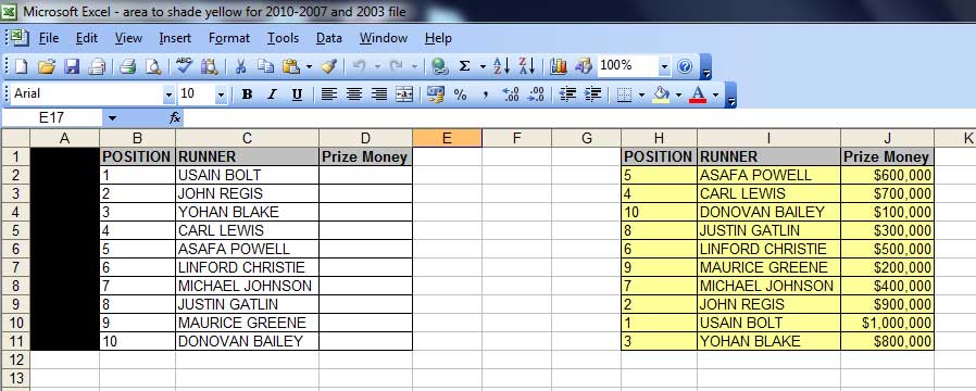 If you want to actually test out the instructions below with exactly the same data in Excel, then we have included a link to the file with the data here –
vlookup specimen file – Usain Bolt, etc.
STEP 1
First, click into cell D2 – as this is where we want the first vlookup result to appear.
STEP 2
Click on the ‘fx’ button above column B – many people start by typing “=vlookup…” but you don’t have to! Clicking the “fx” button is much quicker!
(you will see the ‘Insert Function’ table pop up – screenshot below)
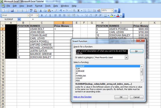
From this window, we will select the vlookup function, as it is one of the ‘most recently used’ functions in the category here.
If the vlookup function isn’t one of the ‘most recently used’ functions, then change the “Or Select a Category” field to ‘All, then scroll to the bottom, where you will see the word ‘vlookup’ and click on it.
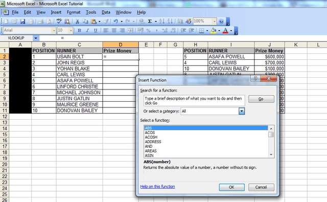
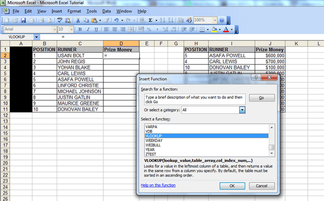
Click ‘ok’ and the function arguments window will pop up. This table will show the Syntax (a fancy word for the format of the formula) and it will display the different parts of the syntax ie VLOOKUP(lookup_value,table_array,col_index_num,range_lookup)
STEP 3
Here, you should click into cell ‘B2’ because that’s the first number or reference for which you want to lookup a value. The ‘look up value’ is the corresponding value we want to find in the first column of the second table – so we want to find out what ‘Prize Money’ the runner in position 1 got in the table that spans columns H to J.
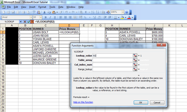
STEP 4
Now click in the next field, the ‘table array’ field (the table array consists of two or more columns of data and the first column in the table array – in this case col. H – has the corresponding numbers that the ‘lookup value is looking at ie the runner positions in this case).
STEP 5
After clicking in the ‘table array’ field, you then need to highlight the columns that that you want to look up data from; so here, we will highlight columns H to J, because our lookup value column starts from column H in the second table, and the Prize Money which we want to check is in col. J
An alternative way to populate the “Table_array” field is to highlight the range of data you’re looking up, starting with your first unique value – in this case cell H2. So you’d highlight cells H2 to J11, because J11 is the last cell in the range. You’d then need to FIX this table array by putting dollar signs in before the H, before the 2, before the J and before the 11, so your formula at the end looks like this: =VLOOKUP(B2,$H$2:$J$11,3,FALSE). If you’re in the table array field and you press F4, then Excel will do this automatically for you. This is useful to know if the spreadsheet doesn’t allow you to highlight cells H to J because some cells are merged or you’re getting an invalid error. But for now, just leave it, ensure, you’re fields look the same as those in the screenshot above then proceed to Step 6, the second last step.
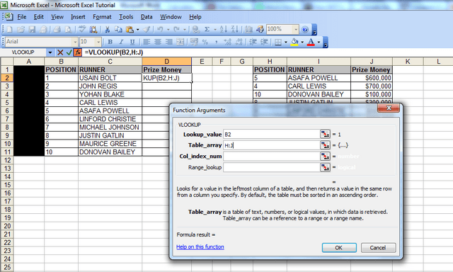
STEP 6
When you highlight the columns, you should note that column J is the 3rd column from column H. We then move onto the next step, Col_index_num, which is the column Index number. Click in that field and type the number 3) – this is because column J is three columns away from column H.
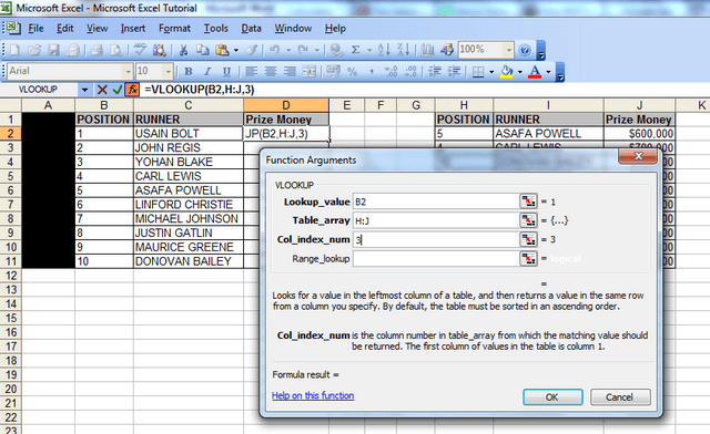
STEP 7
Now, for the last bit, simply click in the ‘range lookup’ field and type in the word false. You should always type in the word false here, because we want the vlookup to return an exact match for what we‘re looking for, and if it doesn’t then we want it to return the word false.
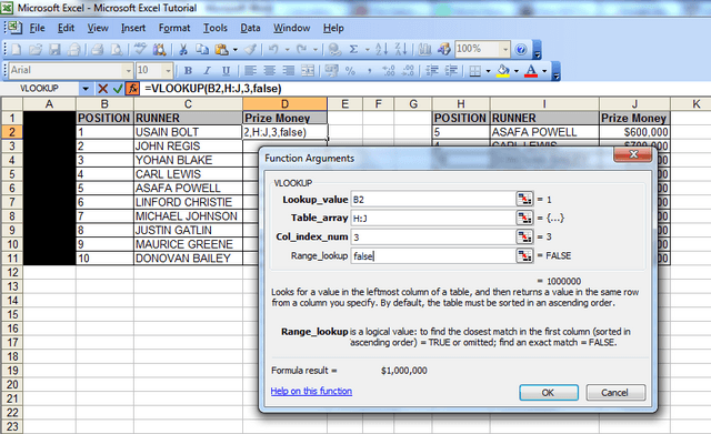
Now click ‘Ok’, and like magic, you will notice that the vlookup has returned the figure of $1,000,000 against Usain Bolt’s name in the first table. If you look at the second table, the figure of $1,000,000 is also against Usain Bolt’s name, so we know the vlookup has worked. And that’s how you string together the vlookup formula in excel.
Now all you have to do is drag down the formula, so that the cells below cell D2 populate, and you save yourself the hassle of manually finding the corresponding Prize Money value for each and every athlete in the first table. In a work scenario, if you had hundreds of rows of data, this would literally save you hours of work!
IMPORTANT point to note – the numbers in the “lookup value” column MUST precede the data you’re looking up! The same is true for the table that you are looking up data from (you must ALWAYS move from the left to the right, when using vlookups!)
Congratulations on finishing the tutorial! If you want to try out a vlookup between two separate workbooks, you can do so here: https://howtovlookupinexcel.com/vlookup-between-two-workbooks
If you want to learn about Pivot Tables, you can do so via this website we created following user demand: http://pivottablesinexcel.com/
If you have problems with your vlookup click here – 13 common problems:
We ask that you take a moment to read our Terms and Conditions and Privacy Policies.
thank you so much man.really appreciate it.
You’re welcome.
I tried changing the name in column I to Jim Regis. =VLOOKUP(B3,H:J,3,FALSE) It still returned the correct value of $900,000. Based upon your comment I was expecting to see FALSE ?
That’s because we’re doing the vlookup using the numbers NOT the names. Vlookups are usually done with numbers. If you want to use the names, you’d need to change the formula to =VLOOKUP(C2,I:J,2,FALSE) as column C has the NAMES.
You are a genious.
Thank you.
Awesome tutorial..I read and read the MS word help for Vloopup and couldn’t figure it out and here in this tutorial after following you pictures..i was able to do it in just 2mintus…truly man you have captured a great tutorial…
Awesome dude , very helpful … 5 star rating
Thanks
gteat tutorial, I got it for 5 min, looked over other instructions for awhile, I coudnt get it;
your help is the great!
Thank you!
Thanks a lot for the insight of excel you have given me.
You’re welcome.
Thanks a lot !!! Saved my day
Really helped a lot, Thank you very much for posting ths
it works perfect … only thing the column where v apply VLOOKUP n get the figures doesnt show the “$” sign in front of the amounts … is that ok in VLOOK UP ?
Yup – you just need to format the currency of the cell to “$”.
Thanks for detailed steps, very useful
Thanks for the good tutorial.
No worries.
Dear Team,
i need your help, could you please let me knpw, i did vlookup, but i am getting #n/a’s, so kindly let me know how to do the vlookup in downloded from SAP or oracle. Thank you
I’d suggest looking at problem number 1 on this page: https://howtovlookupinexcel.com/6-common-problems-with-vlookups
Thank a lot. It really helped me do my task which I was doing in Acess taking lot of time and effort. I believe in Excel.. The best thing of MS Office.
Dude Thanx..phew…job done!!!
No worries.
Very useful information for the users who need to collect the data in different forms
Awesome! I’ve tried the explanation, but it doesn’t work with decimal point. In the table array, I use fraction and decimal point, but the program only recognizes whole nunbers. Is it correct that VLOOK cannot input fraction and decimal numbers other than .50? I use MSWord 2003 and Windows 7 as my OS.
Great job. This is such a useful article. Thanks!
It is simple way to learn difficult things what you have done,sir. it is really help me.
Thanks & regards.
Great example with execution.Thanks
Thanks!
Hi, This is a very effective tutorial. V thoughtfully created. Thanks a lot.
Thanks dude!
Hi,
ThanQ very much…till now I’ve some confusion in tale array and false options in formula…But now its solved…thank U very much…..
Thnx for guide most useful for me
thanks
your explaination is very usfull for me
vijay
The presentation is very simple and crystal clear.Thanks a lot.
This is the best explanation for V-LOOKUP. You are a Legend Mate.
Thanks dude!
Many thanks, very helpful.
Dear Sir,
Thanks for your lesson.
Learnt a lot today.
Thanks,
chea how
Very useful!
Thank you 🙂
You’re welcome!
I checked and tried different answers but this one is the best now i underestand Vlookup
Many thanks
God Bless
Awesome! Thanks!
It’s Very Useful and Clear this..
Thank you so much! This has really helped me. I started a new job and they were trying to explain it to me and I just didn’t get it. This explaination is so simple and easy to understand.
Awesome! Glad I could help!
Very Useful & easy to understand for beginners.
cheers mate!
Thanks
Hi there
This is the best! thank you so much.
Thanks!
Superb, i catch it in just 5 min
THANKS A LOTTTTT. REALLY THE CONCEPT IS EXPLAINED IN VERY SIMPLE MANNER. VERY EASY TO UNDERSTAND AND APPLY.
REGARDS
Thank you so much. It was very clear
thank u ! very much