“This is the quickest I have come across!!!! You are a big help.” Ron
Do you hate going home late?
Do you want to make your job easier?
If you answered yes to either of these questions, then read on.
But before we proceed, many of you have been asking for a step by step tutorial on Pivot Tables, which is now here: Pivot Tables in Excel.We’ve also launched Working with Numbers.
We’ve also created a video version of the tutorial which you can watch here.
Use this file to go try out what is shown in this free excel video tutorial.
The vlookup is the most useful, yet most mis-understood function in Excel. Learning how to vlookup in Excel 2007/2010/2013/2016 and the Excel version in Office 365 can be very useful.
This is a step by step vlookup tutorial (only 7 steps) suitable for beginners. It’s the quickest and simplest way to do a vlookup! It works in all versions of Excel – Excel 2007, Excel 2010, Excel 2013, Excel 2016, Office 365, etc (you just need to find the fx button above column B as shown in the example below).
LEARN HOW TO USE THE VLOOKUP FUNCTION IN EXCEL AND SAVE YOURSELF HOURS WITH ANALYSIS!!
vlookups are usually done between different spreadsheets, but to make it easier to show how they work, I’ve put the data on to one spreadsheet (see image below).
The tables in the spreadsheet have some of the most famous 100m runners in the world – including Usain Bolt (the World Champion!). The runners are numbered from 1 to 10 in column B (the numbers are for illustrative purposes only).
I’ve put the names of the runners / athletes in column C.
IMPORTANT: You should note that the table on the LEFT HAND SIDE is set in ASCENDING NUMERCIAL order ie numbers 1 to 10.
However, the table on the RIGHT HAND SIDE is arranged in ALPHABETICAL order of the names of the athletes. So the numbers in that table DO NOT go from 1 to 10 in ascending order.
We’ll use the vlookup function to get the ‘Prize Money’ each athlete has won in column J in the second table into column D in the first table.
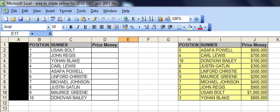 If you want to actually test out the instructions below with exactly the same data in Excel, then we have included a link to the file with the data here –
vlookup specimen file – Usain Bolt, etc.
STEP 1
First, click into cell D2 – as this is where we want the first vlookup result to appear.
STEP 2
Click on the ‘fx’ button above column B – many people start by typing “=vlookup…” but you don’t have to! Clicking the “fx” button is much quicker!
(you will see the ‘Insert Function’ table pop up – screenshot below)
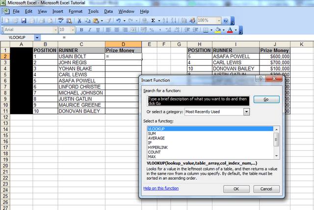
From this window, we will select the vlookup function, as it is one of the ‘most recently used’ functions in the category here.
If the vlookup function isn’t one of the ‘most recently used’ functions, then change the “Or Select a Category” field to ‘All, then scroll to the bottom, where you will see the word ‘vlookup’ and click on it.
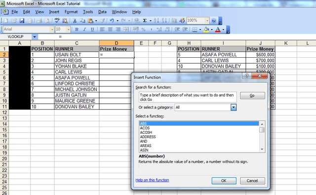
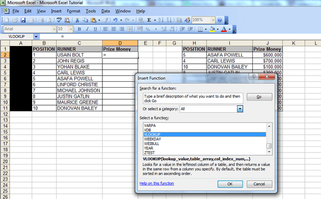
Click ‘ok’ and the function arguments window will pop up. This table will show the Syntax (a fancy word for the format of the formula) and it will display the different parts of the syntax ie VLOOKUP(lookup_value,table_array,col_index_num,range_lookup)
STEP 3
Here, you should click into cell ‘B2’ because that’s the first number or reference for which you want to lookup a value. The ‘look up value’ is the corresponding value we want to find in the first column of the second table – so we want to find out what ‘Prize Money’ the runner in position 1 got in the table that spans columns H to J.
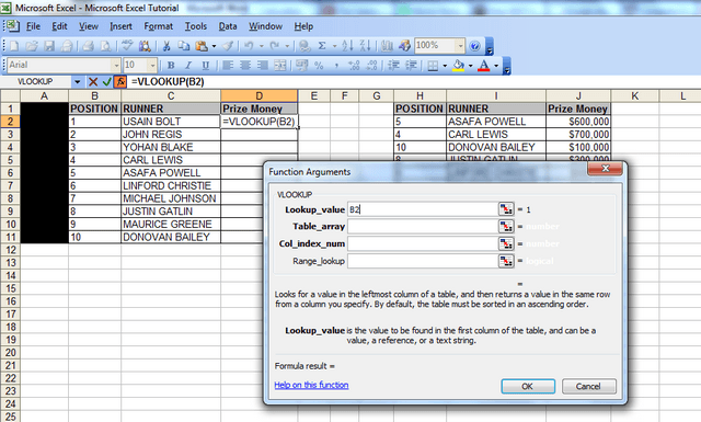
STEP 4
Now click in the next field, the ‘table array’ field (the table array consists of two or more columns of data and the first column in the table array – in this case col. H – has the corresponding numbers that the ‘lookup value is looking at ie the runner positions in this case).
STEP 5
After clicking in the ‘table array’ field, you then need to highlight the columns that that you want to look up data from; so here, we will highlight columns H to J, because our lookup value column starts from column H in the second table, and the Prize Money which we want to check is in col. J
An alternative way to populate the “Table_array” field is to highlight the range of data you’re looking up, starting with your first unique value – in this case cell H2. So you’d highlight cells H2 to J11, because J11 is the last cell in the range. You’d then need to FIX this table array by putting dollar signs in before the H, before the 2, before the J and before the 11, so your formula at the end looks like this: =VLOOKUP(B2,$H$2:$J$11,3,FALSE). If you’re in the table array field and you press F4, then Excel will do this automatically for you. This is useful to know if the spreadsheet doesn’t allow you to highlight cells H to J because some cells are merged or you’re getting an invalid error. But for now, just leave it, ensure, you’re fields look the same as those in the screenshot above then proceed to Step 6, the second last step.
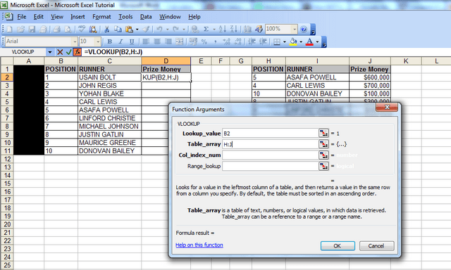
STEP 6
When you highlight the columns, you should note that column J is the 3rd column from column H. We then move onto the next step, Col_index_num, which is the column Index number. Click in that field and type the number 3) – this is because column J is three columns away from column H.
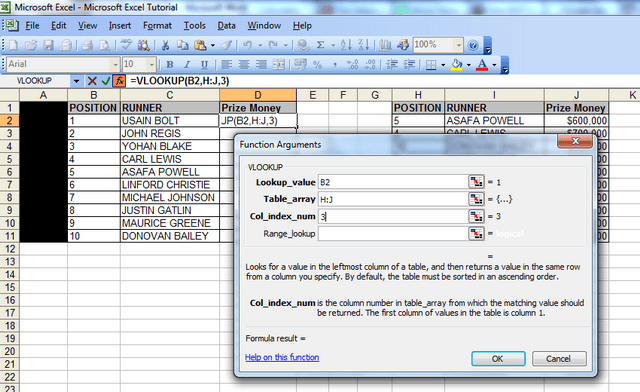
STEP 7
Now, for the last bit, simply click in the ‘range lookup’ field and type in the word false. You should always type in the word false here, because we want the vlookup to return an exact match for what we‘re looking for, and if it doesn’t then we want it to return the word false.
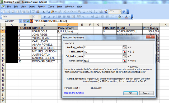
Now click ‘Ok’, and like magic, you will notice that the vlookup has returned the figure of $1,000,000 against Usain Bolt’s name in the first table. If you look at the second table, the figure of $1,000,000 is also against Usain Bolt’s name, so we know the vlookup has worked. And that’s how you string together the vlookup formula in excel.
Now all you have to do is drag down the formula, so that the cells below cell D2 populate, and you save yourself the hassle of manually finding the corresponding Prize Money value for each and every athlete in the first table. In a work scenario, if you had hundreds of rows of data, this would literally save you hours of work!
IMPORTANT point to note – the numbers in the “lookup value” column MUST precede the data you’re looking up! The same is true for the table that you are looking up data from (you must ALWAYS move from the left to the right, when using vlookups!)
Congratulations on finishing the tutorial! If you want to try out a vlookup between two separate workbooks, you can do so here: https://howtovlookupinexcel.com/vlookup-between-two-workbooks
If you want to learn about Pivot Tables, you can do so via this website we created following user demand: http://pivottablesinexcel.com/
If you have problems with your vlookup click here – 13 common problems:
We ask that you take a moment to read our Terms and Conditions and Privacy Policies.
Thank’s a lot very useful.
I’ve learned something new today, thank you! The steps were very simple and understandable. I had one issue, which was in the final step: “drag down the formula, so that the cells below D2 populate”. When I did this the formula changed the range of data cells. ie: b2,H2:j11,3, false, then the next cell would be b3,H3:J12,3 false, etc. What have I done wrong?
Hi Jules
If you send me the file with the formula that you created, I’ll correct it and send it back to you.
I’ve been on holiday – hence the delay, but I’m back now.
Analyst
Hi
Really could do with some help. I have a spreadsheet where I have listed all the staff that have had training. Each of these staff need a refresher every 1 or 3 years. I am now trying to do a summary tab off my spreadsheet so that the Managers know when to book the training courses.
Any chance I can email you the spreadsheet so you can have a look?
Regards…Paresh
Hi Paresh
If you send anonymous data with 2 lines, I can put together a solution for you.
Please don’t send the file if it has any confidential data. I’d advise you to create something similar which has different data, then I can look at it.
Analyst.
I want to get values in column “I” in workbook “A” matching column “B,C,&D” in the same workbook to Workbook “B”
I’d need to see your file. If you send a file with sample data, I can assist.
How do I look up for name list of 1 worksheet and match up with another worksheet using VLOOKUP? Can show me the formula?
Hi Raymond
I can show you the formula if you send me a file with an example of what you’re trying to do.
Hi, this function is very easy when I am working on normal tables. However if I am converting normal table to “Format as Tables” option, I am not able to execute the same formula. Hope you understood my question.
Hi
I don’t think you should have a problem when changing the format. I’d need to see your file. If it doesn’t have confidential info, send it to the email address that you get this response from.
Amazing, Superb, wonderful…I always found Vlookup so hard but u have made it amazingly easy Kudos!!
Great, thanks Divya. Glad I could help.
Hi,
could you maybe help me with a formula for this:
look up value from main table in table 1 and in table 2, if 2 values found then sum up, if 1 value found then give value…
would be pretty awesome…it`s killing me 🙁
Hi
I’ve emailed you directly.
your bit.ly link is not working…
https://howtovlookupinexcel.com/url
Hi Peter
Thanks for bringing that to my attention. The link is fixed now.
Analyst
easy and clear to understand for a fresher.
thanks..!!
very nice:-)
thanks ……
very powerful
Thanks.
This is a nice tutorial… very helpful
Thanks Kezi.
This tutorial was very helpful. Thank you.
Very helpful
Hello Team,
This is really very helpful and easy to learn
I really Appreciate the efforts taken up by the team in helping the students to learn excel easily
Thank you
Thanks Moin. It’s a one-man band at the moment, but thank you!
Big thank you! Very helpful!
I used C2 as the Lookup value rather than B2
It also worked.
Would you say it is just the performance difference perhaps? I mean using numeric value rather than alphanumeric value would ensure faster result from my pc’s point of view, perhaps?
Hi Jaekoo
Apologies for the delay in responding. I have been busy, then ill.
Regarding your question, yes, it is possible to do it with C2 – it sounds like you did it using the words rather than the numbers. Most people use numbers when they’re using vlookups, which is why I’ve explained the formula using the numbers rather than words.
I wouldn’t say it’s a performance difference – it’s just a different way of using the function, which will work on an PC. Hope that helps. Let me know if you still have any questions.
No problem. I am sorry to hear that you were under the weather. Hope all is well on your end now. =)
Please keep up the excellent work. Way to go! =)
Yes, much better now, thanks.
This was very helpful, the MS help version was like trying to read latin. Some better terminology and more detailed instructions would sure help those of us that use this function rarely.
Usually I am matching multiple data from multiple tables and use Access, but this is nice to have when doing simple look up
Hi Scott
Ha ha! I agree re the MS help being complicated.
Glad the content here could help. Let me know if you want me to cover anything else.
Analyst.
thanks a lot…
You’re welcome.
Explained in a very simple and effective manner.
Thanks and Merry Christmas. May Jesus bless you and family.
God bless.
Thank you. Merry Christmas to you too!!
very helpfull thanx…
This is a good way to learn, thank you so much.
Hello Team,
Thank you for the brief explanation on this topic. I have an excel where i would like to use Vlookup formula in a different way. Please look if you can help me.
Emp-ID Salary-Jan Salary-Feb Salary-Mar Salary-Apr
111 10 20 30 40
222 10 20 30 40
333 10 20 30 40
444 10 20 30 40
I have to get the value here
Emp-ID Salary-Apr
444
222
I dont wan’t to use vlookup formula this way eg.=vlookup(A2,TABLEName,Indexname,false), since on my original sheet i don’t know where is my coloumn located, insted of using the column index name is there a way i can match the value and get the data?
Hi
Sorry, but it will be really difficult to answer your question without seeing your sheet. You say that on your original sheet, you “don’t know where your column is located.” I can’t really answer the question, as the details are too vague. But, assuming your info isn’t confidential, I can look at the file to understand the problem further.
Thank you. I used to use this formula daily years ago and this was a great refresher! Saved me lots of time.
No worries. Thanks for the compliment.
Thanks a Lot
It was Easy,quick
& Helpful
You’re welcome.
I am glad, it was great help for me. My sincere thanks
can we take 3 columns in value
I assume you mean the sum of three columns? If so, yes, but I’d recommend that you simply insert a column which is the sum of the three columns that you want then look up that column.
Great. I always found vlookup very difficult and always used to forget it. Now this write up has fixed it. fx function idea and reason to put false is superb.
simpleeeee Superb…
Thanks
OOHHOO……….. THANK U DEAR…. (Y) 🙂
Wow. That was easy. You just saved me a 2 hour meeting with my boss to “learn” this I got it IN MINUTES!!!!!
Thank you!
You’re welcome.
Execellent ThankYou.
THANK U SO MUCH BRO I LEARNED IT QUICKLY WITHIN A MINUTE
THANK YOU SO MUCH…
No worries.
Thanks a ton..its really very helpful..
Very clear guidelines. Able to understand and learn the principle. 🙂
Good, clear instructions. I’ve always found Vlookup a bit confusing but this has helped greatly…Thank you
Awesome! Thanks for the compliment.
it is very useful
Explained so perfectly! Even preempting questions someone may have along the way. Great tutorial! Many Thanks…
Thanks so much for explaining how to use vlookup function, it really gives a perfect answer.