“This is the quickest I have come across!!!! You are a big help.” Ron
Do you hate going home late?
Do you want to make your job easier?
If you answered yes to either of these questions, then read on.
But before we proceed, many of you have been asking for a step by step tutorial on Pivot Tables, which is now here: Pivot Tables in Excel.We’ve also launched Working with Numbers.
We’ve also created a video version of the tutorial which you can watch here.
Use this file to go try out what is shown in this free excel video tutorial.
The vlookup is the most useful, yet most mis-understood function in Excel. Learning how to vlookup in Excel 2007/2010/2013/2016 and the Excel version in Office 365 can be very useful.
This is a step by step vlookup tutorial (only 7 steps) suitable for beginners. It’s the quickest and simplest way to do a vlookup! It works in all versions of Excel – Excel 2007, Excel 2010, Excel 2013, Excel 2016, Office 365, etc (you just need to find the fx button above column B as shown in the example below).
LEARN HOW TO USE THE VLOOKUP FUNCTION IN EXCEL AND SAVE YOURSELF HOURS WITH ANALYSIS!!
vlookups are usually done between different spreadsheets, but to make it easier to show how they work, I’ve put the data on to one spreadsheet (see image below).
The tables in the spreadsheet have some of the most famous 100m runners in the world – including Usain Bolt (the World Champion!). The runners are numbered from 1 to 10 in column B (the numbers are for illustrative purposes only).
I’ve put the names of the runners / athletes in column C.
IMPORTANT: You should note that the table on the LEFT HAND SIDE is set in ASCENDING NUMERCIAL order ie numbers 1 to 10.
However, the table on the RIGHT HAND SIDE is arranged in ALPHABETICAL order of the names of the athletes. So the numbers in that table DO NOT go from 1 to 10 in ascending order.
We’ll use the vlookup function to get the ‘Prize Money’ each athlete has won in column J in the second table into column D in the first table.
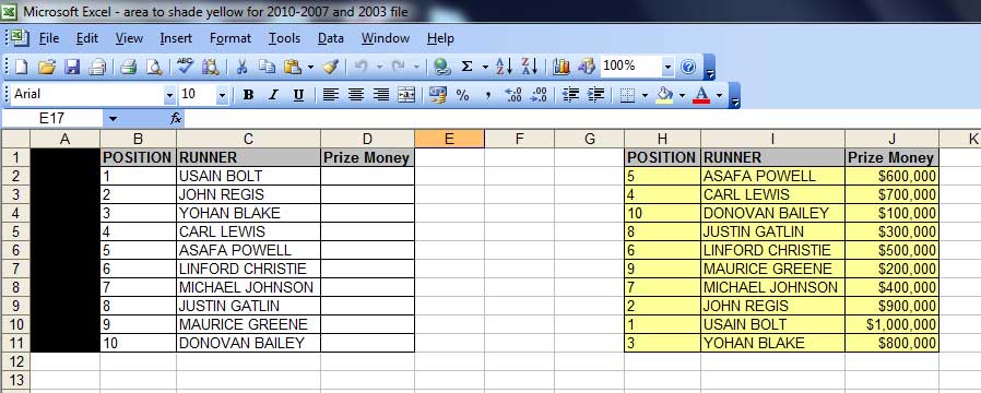 If you want to actually test out the instructions below with exactly the same data in Excel, then we have included a link to the file with the data here –
vlookup specimen file – Usain Bolt, etc.
STEP 1
First, click into cell D2 – as this is where we want the first vlookup result to appear.
STEP 2
Click on the ‘fx’ button above column B – many people start by typing “=vlookup…” but you don’t have to! Clicking the “fx” button is much quicker!
(you will see the ‘Insert Function’ table pop up – screenshot below)
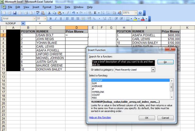
From this window, we will select the vlookup function, as it is one of the ‘most recently used’ functions in the category here.
If the vlookup function isn’t one of the ‘most recently used’ functions, then change the “Or Select a Category” field to ‘All, then scroll to the bottom, where you will see the word ‘vlookup’ and click on it.
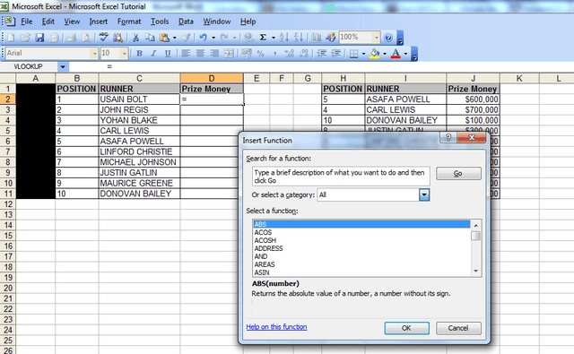
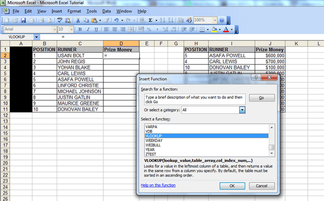
Click ‘ok’ and the function arguments window will pop up. This table will show the Syntax (a fancy word for the format of the formula) and it will display the different parts of the syntax ie VLOOKUP(lookup_value,table_array,col_index_num,range_lookup)
STEP 3
Here, you should click into cell ‘B2’ because that’s the first number or reference for which you want to lookup a value. The ‘look up value’ is the corresponding value we want to find in the first column of the second table – so we want to find out what ‘Prize Money’ the runner in position 1 got in the table that spans columns H to J.
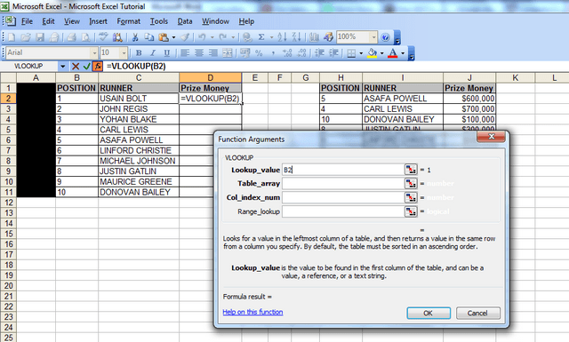
STEP 4
Now click in the next field, the ‘table array’ field (the table array consists of two or more columns of data and the first column in the table array – in this case col. H – has the corresponding numbers that the ‘lookup value is looking at ie the runner positions in this case).
STEP 5
After clicking in the ‘table array’ field, you then need to highlight the columns that that you want to look up data from; so here, we will highlight columns H to J, because our lookup value column starts from column H in the second table, and the Prize Money which we want to check is in col. J
An alternative way to populate the “Table_array” field is to highlight the range of data you’re looking up, starting with your first unique value – in this case cell H2. So you’d highlight cells H2 to J11, because J11 is the last cell in the range. You’d then need to FIX this table array by putting dollar signs in before the H, before the 2, before the J and before the 11, so your formula at the end looks like this: =VLOOKUP(B2,$H$2:$J$11,3,FALSE). If you’re in the table array field and you press F4, then Excel will do this automatically for you. This is useful to know if the spreadsheet doesn’t allow you to highlight cells H to J because some cells are merged or you’re getting an invalid error. But for now, just leave it, ensure, you’re fields look the same as those in the screenshot above then proceed to Step 6, the second last step.
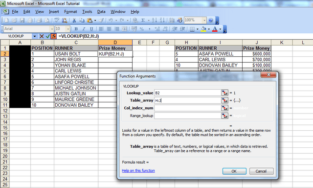
STEP 6
When you highlight the columns, you should note that column J is the 3rd column from column H. We then move onto the next step, Col_index_num, which is the column Index number. Click in that field and type the number 3) – this is because column J is three columns away from column H.
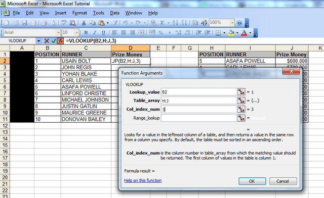
STEP 7
Now, for the last bit, simply click in the ‘range lookup’ field and type in the word false. You should always type in the word false here, because we want the vlookup to return an exact match for what we‘re looking for, and if it doesn’t then we want it to return the word false.
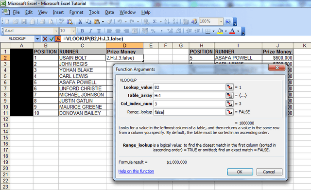
Now click ‘Ok’, and like magic, you will notice that the vlookup has returned the figure of $1,000,000 against Usain Bolt’s name in the first table. If you look at the second table, the figure of $1,000,000 is also against Usain Bolt’s name, so we know the vlookup has worked. And that’s how you string together the vlookup formula in excel.
Now all you have to do is drag down the formula, so that the cells below cell D2 populate, and you save yourself the hassle of manually finding the corresponding Prize Money value for each and every athlete in the first table. In a work scenario, if you had hundreds of rows of data, this would literally save you hours of work!
IMPORTANT point to note – the numbers in the “lookup value” column MUST precede the data you’re looking up! The same is true for the table that you are looking up data from (you must ALWAYS move from the left to the right, when using vlookups!)
Congratulations on finishing the tutorial! If you want to try out a vlookup between two separate workbooks, you can do so here: https://howtovlookupinexcel.com/vlookup-between-two-workbooks
If you want to learn about Pivot Tables, you can do so via this website we created following user demand: http://pivottablesinexcel.com/
If you have problems with your vlookup click here – 13 common problems:
We ask that you take a moment to read our Terms and Conditions and Privacy Policies.
Just wanted to say thanks for the vlookup video – it was so easy to follow & has helped me immensely. Thank you so much
That’s great to hear and thank you for the feedback, Mirella.
If you have any questions, let us know.
This was really easy to learn with this step by step guide. I have a job interview tomorrow and will be tested on this so I appreciate the assist 🙂
Awesome! That’s great to hear.
Glad we could help! If you have any other questions, let us know.
I am still a bit confused. I am making an invoice that will autofill. I have the invoice on one sheet, clients in another sheet and the products on another sheet. I’ve gotten the products to autofill but not the clients. I would like to be able to enter an account number then their name, address, phone and email to auto populate. I’ve entered what I thought was correct but it either comes up with a n/a or it goes hunting for a another worksheet! What am I doing wrong.
Hi PJ
Can you create a dummy file with one row with the incorrect result and send it through?
Analyst
Thank you very much. This really helped me to learn esp. with same sample sheet able to download and follow the steps.
You’re welcome. 🙂
My workbook is fairly complex. I followed your step by step but I keep on getting N/A
Hi Shireen
Are you doing a vlookup within a single sheet, two different sheets, or different workbooks?
And have you tried the alternative method explained in Step 5 here? https://howtovlookupinexcel.com/vlookup-between-two-workbooks/
Your workbook may have merged cells which could be causing the issue. If so, then the alternative method mentioned above should work.
Let me know if not.
Analyst
Hi,
You are getting that because you did not lock the table array. Press f4 to lock the table array H:J and try again.
Amon – you don’t have to lock the table array for the vlookup to work.
There are several ways to do vlookups, and I describe a method which doesn’t require you to lock the array on this site.
There could be several reasons why Shireen was getting #N/As -I’ve covered 5 different #N/A errors here: https://howtovlookupinexcel.com/13-common-problems-with-vlookups/
So without seeing her file, you can’t possibly say for certain which #N/A error it is.
I have done vlookup things.
but when I send the same vlookup file to anyone,they are not able to see the correct name.They only have #NA in the excel sheet.
Pl suggest.
Hi Piyush
That’s a strange problem that I’ve never heard of!
However, if the calculation in their Excel format is set to manual instead of automatic, that could be the cause of the issue.
Let me know if that helps?
Analyst
🙂 OK !
This info was very helpful…. thanks
No problem! Glad you found it useful!
Thank you!
Really helpful.
Thanks.
Sir i can’t apply the formula for matching the from one sheet to another..
You haven’t clarified whether you’re using your own file or the sample file provided on this website.
This was very helpful and very easy to follow.
Thank you. That’s good to know!
I am setting up a vlookup to get me the closest value of a percentage or a dollar amount. Each time I run the system, I get an incorrect return. It gives me the last possible value in the column. I am assuming it is because there is not an exact value. I need to be able to calculate the dropoff of Mortgage insurance, and it drops off automatically after 78%. I want this to give me the payment number the LTV drops below 78%. It always gives me 360 payments. It should be giving me 114 or 115.
Hi Cory
It sounds like your formula may be incorrect.
But without seeing your file, I can’t tell.
If you can send dummy data to the email address that you get this response from, I can assist further.
Analyst
THANK U SIR
You’re welcome.
I have two sets of data and managed to use vlookup to return the correct information. However, when there is not a match on some items, which I expected, the formula returns #N/A. How can I get it to return a blank cell, or nothing?
You need to add *=iferror(* at the beginning and *,””)* at the end (excluding the stars).
It’s covered under the “New Update” section under problem 10 on this page: https://howtovlookupinexcel.com/13-common-problems-with-vlookups/
Just put down two inverted commas ie “” instead of the zero described in the update, if you want to return a blank.
Thanks for the great tutorial. Can you use VLOOKUP function and skip columns in the table array? My table array will be to the right of the lookup value, but I don’t need data from each column.
Hi John
You certainly can.
You just need to make sure your table array covers all the columns you want to look up, then select the relevant “col_index_num” or column index number.
If you need more detail, let me know.
Analyst
Been ignoring this function for long. This made it easy to understand and use it quickly. Thanks !
Thank you that was very helpful
You’re welcome.
Brilliant….now I finally understand how Vlook up works!
i liked the idea its very great but i have a question though, suppose in your given example i only had positions that means i only have numbers so if i type “1” in position column then name of runner and his respective prize should be shown can that be done?
thanks for reading it
Hi
I’m not sure why you’d want to manually type in numbers – the point of it is to automate the process.
But, yes, you’d just have to do a vlookup with the two columns you’ve described – position and runner.
Analyst
how can i do a vlookup with the two columns that’s what i wanted to know sir because i tried but there was some sort of syntax error.
Send me the file with the syntax error that you got.
Analyst,
Igot the formula worked out in the first column in the sample demo filed you provided.
But I don’t know how I can drag the formula in rest of the columns. I tried to copy & paste the formula but it did not work.
Can you please guide me? Thank you so much,
Vijay
Hi
To drag the formula down the column, all you need to do is hover over the cell until you see a black cross, then drag it down.
Analyst
Hello,
Thank you. Very simple and easy to understand. It just took 5 mins as you indicated 🙂
That is awesome, Sam! Glad to hear that the tutorial helped!
I have two worksheets with a matching ID code for our employees. One sheet tracks all our employees and there relevant data. The other simply tracks the hypos and what school they graduated from. If they had multiple schools, the ID code is listed for each school they graduated from. I have been able to use Vlookup to add the school to the master spreadsheet. The issue I have is that some of our employees got a BS from one school, Masters from another and a doctorate from another. Vlookup only gives you the last match. How can I get it to add all the schools listed?
Hi Walter
I haven’t seen your spreadsheet, so I can only make assumptions here. If an employee has been to more than one school and the schools are listed in separate rows, then it won’t be possible to use the vlookup to return different results for each school.
You may be better off doing a pivot table. If you send dummy data, I can have a look for you. But please only send info if it is NOT confidential and you have permission to do so.
Rgds
Analyst
thank you sir i learnt much needed vlookup for my job
You’re welcome Sandeep.
Great work and many thanks. This is the best tutorial have I come across on Vlookup and Pivots. Are there other Excel tutorials from you?
Hi Clarence
Thanks for the feedback – it’s much appreciated.
I don’t have any other tutorials, at present, but will let you know if and when I do create some additional ones.
Analyst
Is there a free tool one can download to “annonymize” Excel data? I have a large spreadsheet but can not “annonymize” the data manually, as there is too much.
Thank you.
Hi David
I did a quick search on google but couldn’t find anything quick and simple.
What’s the issue you have? If you send a copy of the sheet with two rows and dummy data, ensuring you remove anything confidential, I can have a look.
Analyst
I ended up using this to anonymize the data:
http://www.codematic.net/excel-tools/excel-anonymiser.htm
It still only partially worked for what I needed. I also had a bunch of names I needed to change, so I used search and replace to change much of the names and between that worked for me.
My question is actually not a vLookup question, but a pivot table question. But I asked you as I see you frequently tell people to anonymize the data. Thanks for your help!
Yes, I came across that site as well, but the macro was written for Excel 2003 and earlier versions, and they said it doesn’t work properly for later versions. I thought you may be using Excel 2007 or 2010, as 2003 is quite old now.
What’s the question you have about pivot tables?
how to use vlookup function in excel window 2007. i want to compare tally export data & excel sheet data to
compare. how to use it
Hi Alka
I’m not sure exactly what your question is.
If you can send dummy data, then I can assist.
Analyst
Thanks for the vLookup and Pivot tables step and process. I’ll put this into good use :). Do you have any materials on Macros?
Thanks again!
Hi Rick
I don’t have any material on macros yet, but I’ll let you know when I do.
Analyst
Hi. I am looking for help with a formula in Excel. I have a spreadsheet with many worksheets. Each worksheet contains a document copied into it with tables, sentences, and paragraphs. I have a list for words and numbers in the first worksheet that I need to find in all the others. I am using “IF(ISERROR(VLOOKUP($E16,’148N’!$B$7:$E$5000,1,FALSE)),””,”Yes”) but it is only finding the word at E16 if it is NOT in a sentence and only if it is in Column B (it will not search Column C in tab #148N for that same word. Can you assist? Is vlookup the correct formula for this situation?
Hi Kate
Apologies for the delay in responding.
From what you’ve described, the formula does not appear to be correct.
For example, you don’t need a dollar sign after the bracket after the word “vlookup” in the formula.
Also, is the tab you’re looking up the data from called “148N”? That’s a very unusual name for a tab. If it’s not called that, then that’s another thing that you’d need to correct with the formula.
To give you the correct formula, I’d need to be able to see the spreadsheet, as I don’t know the range of data that you’re looking up.
However, you’d need to create dummy data, if the data is confidential – if you can create dummy data for, say, 5 rows, I can give you a steer.
Analyst
THANKS A TON…!
You’re welcome.
This was so easy and helpful. Now I am using vlook ups for massive spreadsheets that I maintain at my job. Thank you so much!
Any instructions for “dummies” on pivot tables?
Hi Wendy
Thanks for the feedback.
Yes, I created a tutorial for pivot tables here: http://pivottablesinexcel.com/
Let me know if you have any questions about it.
Analyst
Many Thanks
You’re welcome.
This is the best explanation out there and the fact that you go into all the possible errors is so helpful. I have been trying to create this formula all day and your explanation is the only one I could understand and worked for me.
Thank you very much!
That’s great LY! Glad the site helped!
And thank you for your kind words. If you have any queries, let me know.
Analyst
Vlook-up seemed like rocket science to me after I went through tutorials/videos on youtube! BUT you’ve really done a great job of explaining it! I’ve finally learned to use this function!Thanks a bunch!
That is awesome Amna! I’m really glad my tutorial helped.
Let me know if you have any other questions about it.
Excellent tutorial. Thanks soooo much for your help. Its much appreciated 🙂
Glad it helped you. Thank you for your kind comments.
Analyst
This was a very simple and easy method to follow. Thanks a lot!
Thank you Hem N.
Very clear instructions
Thanks Benson.
Thanks it works
You’re welcome.
INCREDIBLY helpful! Words can’t express my gratitude that you took the time to put this together for everyone. Had never done a Vlookup in my life (but heard horror stories about them) – I had finished what I needed to do in 10 minutes start to finish thanks to this guideline. You have my complete appreciation.
Thank you for taking your time to put this together.
Thanks dude. That’s the nicest testimonial I’ve ever had about the tutorial!
It’s much appreciated.
Thank u soooooooooo much……for making it so easy for us…………
You’re welcome.
can we do a vlookup on names instead of numbers.
like i have a list of names in one column and some numbers in another. I need to get the numbers to another table using the name as reference.
Yes, you can. But using names is less reliable. You’ll need to make sure that the names match exactly for the vlookups to work.
You’re welcome.