Do you want to become a vlookup expert?
Do you want to save time looking up data at work?
If you answered yes to either of these questions, then read on.
The vlookup is one of the most useful, yet most mis-understood functions in Excel.
This tutorial is a 7 step guide where we provide you with a file that you can use to learn how to vlookup between two different sheets in Excel – this works in all versions – Excel 2019, Excel 2016, Excel 2013, Office 365, etc.
Here is the link to the file we use – open this before starting the tutorial: vlookup between two different sheets – file.xlsx
Now that you have the file open, we’ll explain what’s in it, so you understand the context:
There are TWO worksheets in the file. Both contain a list of products which the majority of people would buy in a supermarket – Milk, Bread, Jam, etc.
However, only one sheet contains a list of prices which we’ll use the vlookup to get into the other sheet.
We’ll use the vlookup function to get the prices of the food data from the “worksheet with prices” tab into the “worksheet without prices” tab.
Step 1
Before you start, open the file from this site AND make sure you’ve clicked the “Enable editing” button (see screenshot below) then save it to your Desktop, otherwise any changes you make won’t work!

Screenshot of the ‘Enable Editing’ button in Excel, when you open the file.
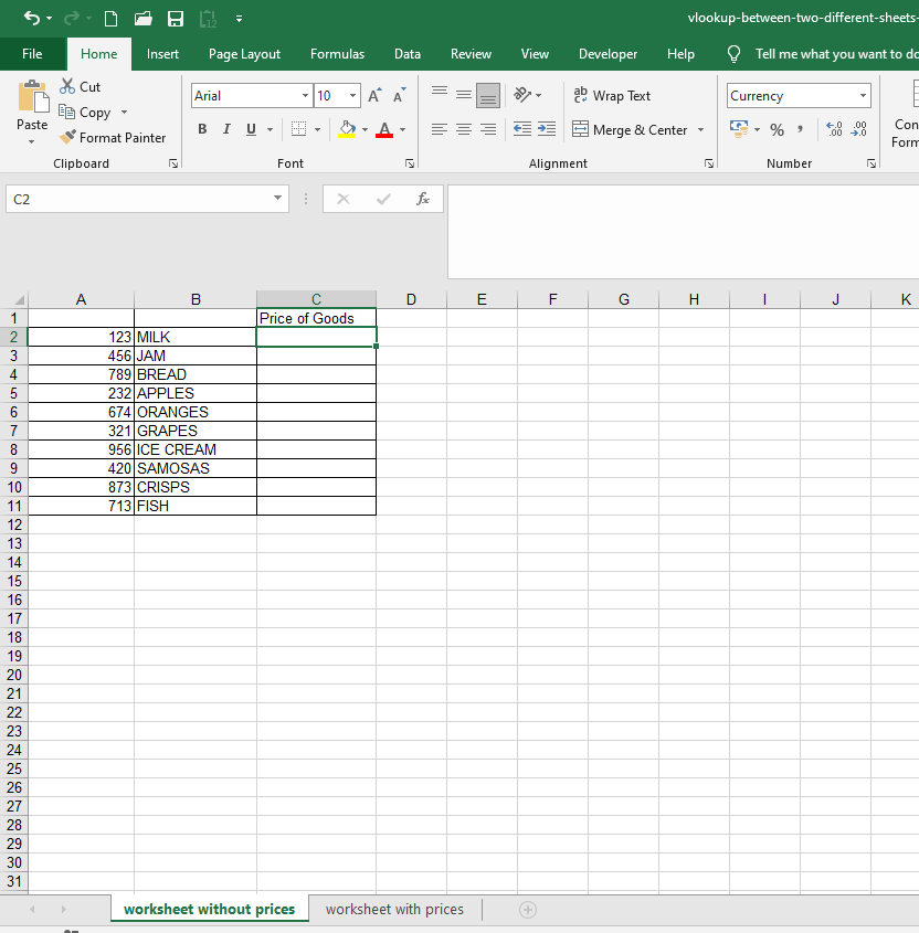
When you open the file (“vlookup between two different sheets”) you will see the screen below. Column C in the “worksheet without prices” tab is where we will pull in the “Price of the Goods” from the “worksheet with prices” sheet. Cell C2 in the “worksheet without prices” tab should already be selected, as that’s where we want the first result to appear.
Screenshot of what the file looks like, when you open it.
Step 2
Click on the “fx” button which is above column D (see screenshot below). The ‘Insert Function’ window will then show up (also shown in the screenshot below). If the “vlookup function” is already selected, like in the screenshot below, click “ok”. If it’s not, the text below this screenshow will show you what to do next.
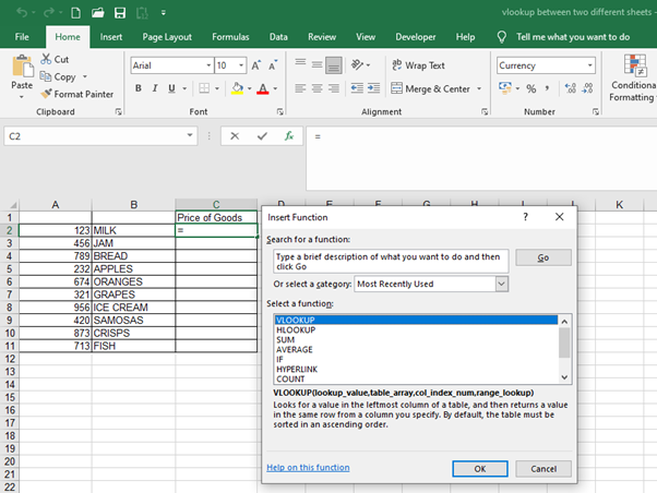
Screenshot of the Insert Function window with the list of the Most Recently Used functions.
If the “vlookup function” isn’t already selected, then in the “or select a category” field shown in the screenshot above, change the option in the drop-down from “Most Recently Used” to “All” then scroll down until you get to the vlookup function, as shown in the screenshot below.
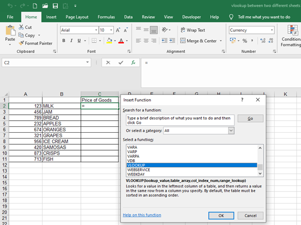
Screenshot of the Insert Function window with ‘All’ selected under the ‘Or select a category’ field.
Once you’ve selected the “vlookup function” from the drop-down menu and clicked ok, the “Function Arguments” window will appear.
Step 3
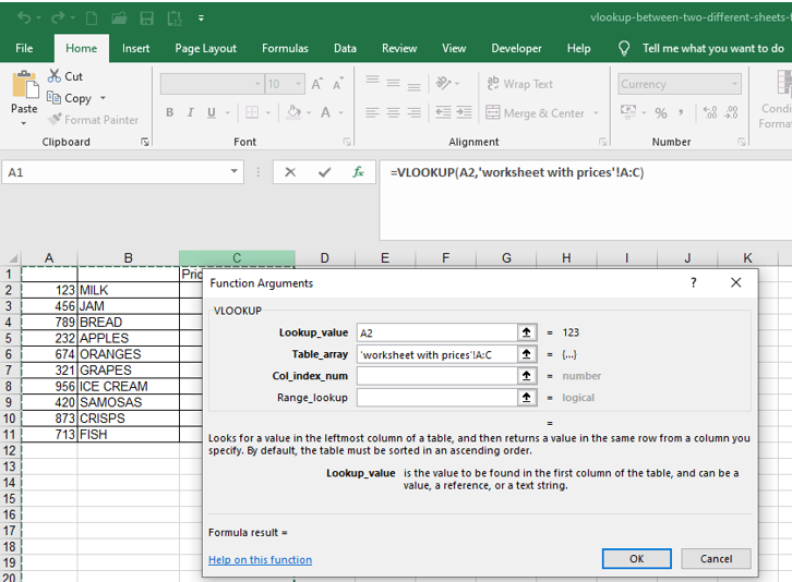
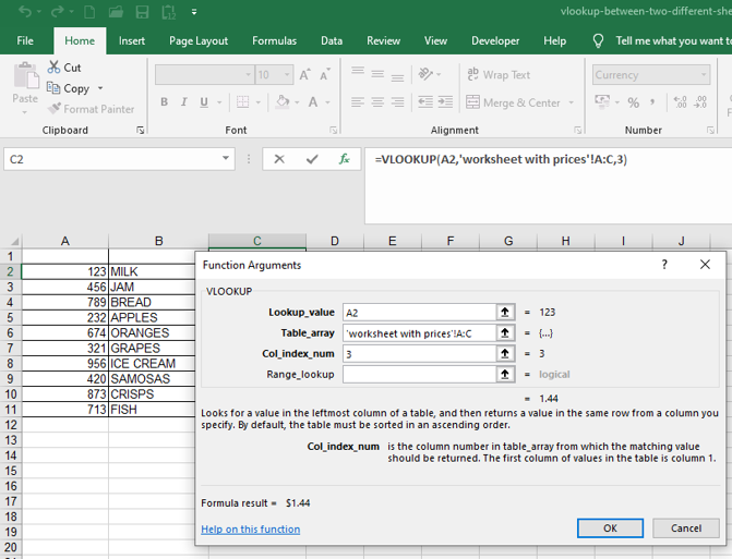
The “Function Arguments” window will show 4 different fields which need to be populated for the vlookup to work. For the first field, the “Lookup_value”, click on cell A2, as illustrated in the image below. It has green dotted lines around it in the screenshot below.
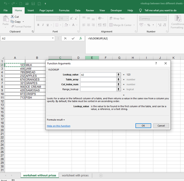
Screenshot showing the vlookup Function Arguments window for the vlookup function. Cell A2 has been selected for the ‘Lookup_value’ field.
Step 4
Now click into the “Table_array” field, which is the field below the ‘Lookup_value’ field (see the screenshot above). A “table array” is a fancy phrase for describing two or more columns of data in Excel.
We’ll populate the data for this field in Step 5.
Step 5
This part is where the other worksheet comes in! After you’ve clicked in the “Table_array” field, click into the other worksheet (“worksheet with prices”) and highlight columns A – C in that worsheet.
We highlight columns A – C in that worksheet because column A has the “Lookup_value” that is in the “worksheet without prices” and column C has the “Prices” that we want to get.
When you highlighted columns A – C, you may have noticed that the characters “3C” appeared at the top of column E – this is a quick way of Excel telling you how many columns there are in the data you’ve highlighted – it saves you having to count the columns manually, which a lot of people in offices do! If you didn’t notice that, clear the data in the “Table array” field and highlight columns A – C again in the “worksheet with prices” tab but ensure you hold don’t release the mouse key, when you’re highlighting the columns, because as soon as you release it, the “3C” will disappear.
Many office workers don’t know this trick and waste a lot of time manually counting the columns! But we’re here to save you time!
Your screen should now look like this:
Screenshot of the vlookup Function Arguments window with columns A – C highlighted.
NB – an alternative, but IMPORTANT way to populate the “Table_array” field is to highlight the range of data you’re looking up, starting with your first unique value – in this case cell A2. So you’d highlight cells A2 to C11, because C11 is the last cell in the range. You’d then need to FIX this table array by pressing F4 on your keyboard or ‘fn and F4’ at the same time if you have an HP laptop. Pressing F4 automatically adds in dollar signs, to fix the range of data your analysing – once pressed, “Table_array” field should look like the screenshot below ie a dollar sign before the letter A, before the number 2, before the letter C and before the number 11:
Screenshot showing an alternative way to populate the ‘Table_array’ in the vlookup Function Arguments window. Columns A2 to C11 have been highlighted and the range has been fixed ie dollar signs have been added.
This is useful to know if a spreadsheet doesn’t allow you to highlight columns A to C because some cells are merged or you’re getting an invalid error. But for now, just clear everything in the ‘Table_array’ field, then highlight columns A-C again in the ‘worksheet with prices’ tab. Your screen should now look the same as the screenshot below.
Screenshot of the vlookup Function Arguments window with columns A – C highlighted.
And you can now proceed to Step 6, the second last step.
Step 6
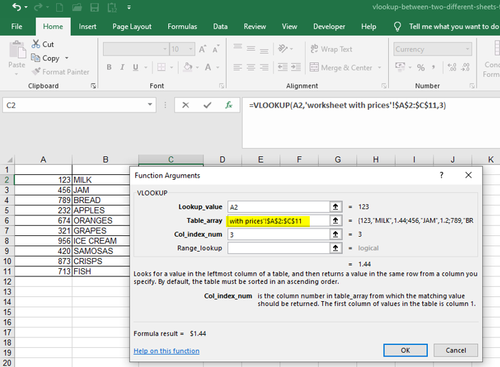
Click into the “Col_index_num” field – you will notice that your screen returns back to the first worksheet, the “worksheet without prices” – don’t panic! All you have to do here is put in the number 3 in the “Col_index_num” field shown in the screenshot below.
We put in the number 3 here because column C in the “worksheet with prices” has the prices of the goods that we want and it is three columns away from column A, which has the unique lookup values that we are using. Or if you noticed the “3C”, it means “3 columns” so you know you have to insert the number 3 in the “Col_index_num” field. A screenshot of how everything should look so far is below.
Screenshot showing the ‘Col_index_num’ field with the number 3 in the vlookup Function Arguments window.
NB if you get an error like the one in the screenshot below, it means that you’ve accidentally clicked on the ‘worksheet without prices’ tab twice or clicked on something which has resulted in additional text appearing in the ‘Table_array’ field – in the screenshot below, the text ‘worksheet with prices’! (highlighted in yellow) appears twice, which is what’s causing that error.
The solution here is to just clear everything in the ‘Table_array’ field then ensure that you’re still in the ‘worksheet with prices’ tab, then highlight cells columns A – C again.
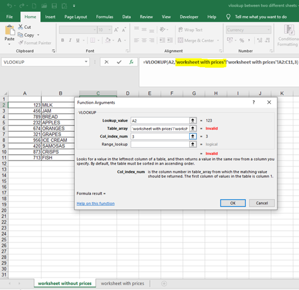
Screenshot showing how the ‘invalid’ error can happen, when creating the vlookup function.
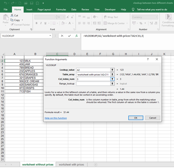
To recap, your screen should look like this before proceeding to the last step (Step 7)
Screenshot showing how the vlookup Functions Argument window should look before proceeding to the last step (Step 7).
Step 7
The final step! Click into the ‘range lookup field’ and type the word ‘FALSE.’
Now click ‘OK’ and, like magic, the formula will return the first result that we’re looking up i.e $1.44.
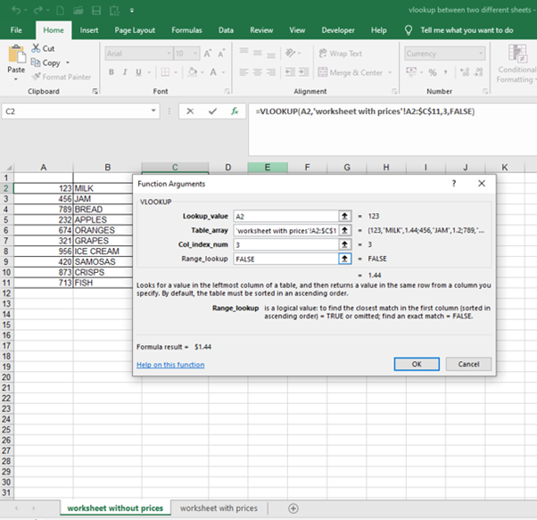
Screenshot showing the ‘Range_lookup’ field populated with the word false.
After that, simply drag down the formula in cell C2 in the “worksheet without prices” and the “prices” of all the other goods from the other sheet will auto-populate.
The word ‘FALSE’ in the ‘Range_lookup’ field ensures that the vlookup only returns an EXACT match. If it doesn’t find an exact match for the ‘lookup value’ we’re using, then it will return an N/A – more about this in the “13 reasons why your vlookup is not working” page mentioned at the end of this.
Your formula in the end should look like this (in cell C2 in the worksheet without prices):
=VLOOKUP(A2,’worksheet with prices’!A:C,3,FALSE)
If your formula does not look like this, then you need to check that you’ve followed the steps above correctly.
And that’s how you do a vlookup between two sheets!
IMPORTANT point to note – the numbers in the “lookup value” column (column A in the ‘worksheet with prices’ tab) MUST precede the data you’re looking up! So in the ‘worksheet with prices’ tab, if the numbers in column A were AFTER the prices in column C, then you wouldn’t be able to use a vlookup.
So with vlookups, you must ALWAYS move from the LEFT to the RIGHT – in this case, when we highlighted columns A – C in the ‘worksheet with prices’ tab, our ‘lookup_values’ started on the left (in column A) and the values we needed were to the RIGHT of column A ie column C.
If you want to learn how to do a vlookup between two workbooks, click here.
If you want to learn about Pivot Tables, you can do so via this website we created following user demand: https://pivottablesinexcel.com/
If you have problems with your vlookup click here – 13 common problems: https://howtovlookupinexcel.com/13-common-problems-with-vlookups/
If you have problems with your vlookup click here– 13 common problems:
We ask that you take a moment to read our Terms and Conditions and Privacy Policies.
Please let me know how I can drag the formula into all the columns. It worked in the first colum.
But I don’t know how I can use the same formula in rest of the columns automatically without entering manually in each column.
Looking forward for your response soon.
I really appreciate your time. Thank you so much.
Vijay
Hi
If you want to drag the formula to separate columns, then you’ll have to fix the column with your lookup values AND fix the range you’re looking up, which is explained in the alternative section in step 5.
It will be just easier to create a vlookup in the new column that you want it to appear.
If you have lots of new columns where you want to create vlookups and your file doesn’t contain confidential information, then send it through and I’ll have a look.
Analyst
Thanks for step 5 — I would get so far and the table array would move as I pasted down the formula.. problem solved.
No problem.
Glad I could help!
Very useful material.. Thanks!!
You’re welcome.
Step 7 gave me the help I needed! Thanks a lot!
You’re welcome.
I am fairly new to excel and was glad you provided this step-by-step. I was able to duplicate this…. thank you so much! I would like to learn Pivot tables…any future training there?
Hi Sheila
Thank you for your comment.
I don’t have content on pivot tables at present, but will definitely let you know if/when I do.
tnx a lot for this tnx a lot for this very helpful! Appreciate your help with the below two fold question:a) what if my worksheet names are not as consistent as in your example ? i.e. instead of region 1, 2, 3 I have alphanum codes such as AB1, DB2, CC3 for worksheet names. is there wild card’ variable make excel look in the next sheet irrespective of its name? b) is there a way to tell excel which is the first worksheet to vlookup into and which is the last ?
Hi Shagow
a) I don’t think so. The worksheet names won’t matter though.
b) Ditto. I believe you’d have to do this manually. Would it not be easier to simply dump all the data you want to lookup in one sheet, instead of having to lookup several sheets?
Very helpful and nicely written. thanks
Thanks Mike. Glad I was able to help!
Thank you.
That was fantastic.
Any slides on Pivotal table ???
Hi Kaddu
I don’t have slides on pivot tables at the moment, but I am working on another site which will cover other functions in Excel – I will look into covering pivot tables as well, but the site is still work-in-progress and I’m not sure exactly when it will launch. If you have any other questions about vlookups in the meantime, let me know.
This is great. Gave perfect step by step instructions for me.
Only mis wording appears to be
in STEP 6: “this is because column J is three columns away from column I” I think you mean column J is the 3rd column in the area you are looking up the data for.
Thanks Suzie – apologies for the delay – you are correct – I have made a slight amendment – it was a typing error!. I meant to write “this is because column J is three columns away from column H” rather than column I. Thanks for your observation, it is appreciated.
thank you for dumbing this down with visuals. I was able to create a vlookup along with you and got it!
That is awesome, Patricia! Glad you got it working!