Do you want to use Excel more efficiently?
Do you want to be able to go home earlier?
If you answered yes to either of these questions, then read on.
The vlookup is the most useful, yet most mis-understood function in Excel.And vlookup in Excel 2007/2010 is very powerful
This is a step by step vlookup tutorial (only 7 steps) suitable for beginners and made more interesting by including Usain Bolt, as it’s the quickest (and simplest) way to do a vlookup!! This method works in Excel 2003, Excel 2007, and Excel 2010 (you just need to find the fx button above column B demonstrated in the example below).
LEARN HOW TO USE THE VLOOKUP FUNCTION IN EXCEL AND SAVE YOURSELF HOURS WITH ANALYSIS!!
vlookups are usually done between different spreadsheets, but to make it easier to show how they work, I’ve put the data on to one spreadsheet in the table in the first image below.
The table has some of the most famous 100m runners in the world. They are numbered from 1 to 10 in column B (the numbers are for illustrative purposes only).
I’ve put the names of the athletes in column C.
IMPORTANT: You should note that the table on the LEFT HAND SIDE is set in ASCENDING NUMERCIAL order ie numbers 1 to 10.
However, the table on the RIGHT HAND SIDE is arranged in ALPHABETICAL order of the names of the athletes. So the numbers in that table DO NOT go from 1 to 10 in ascending order.
We’ll use the vlookup function to get the ‘Prize Money’ each athlete has won in column J in the second table into column D in the first table.
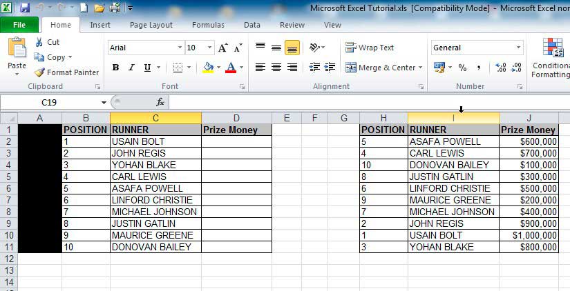
If you want to actually test out the instructions below with exactly the same data in Excel, then we have included a link to the file with the data here –
vlookup specimen file – Usain Bolt, etc.
STEP 1
First, click into cell D2 – as this is where we want the first vlookup result to appear.
STEP 2
Now click on the ‘fx’ button above column B – many people start by typing “=vlookup…” but you don’t have to! Clicking the “fx” button is much quicker!
(you will see the ‘Insert Function’ table pop up – screenshot below)
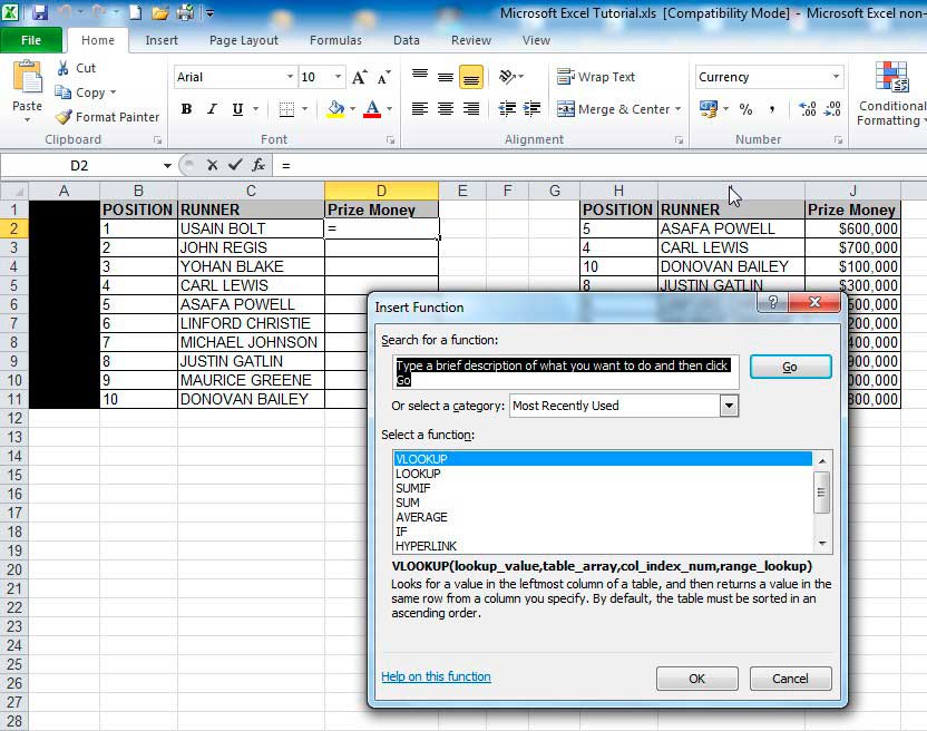
From this window, we will select the vlookup function, as it is one of the ‘most recently used’ functions in the category here.
If the vlookup function isn’t one of the ‘most recently used’ functions, then change the Category to all, select ‘All’, then scroll to the bottom, where you will see the word ‘vlookup’ and click on it.
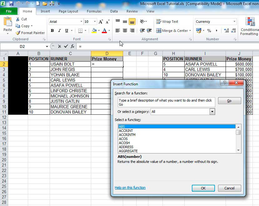
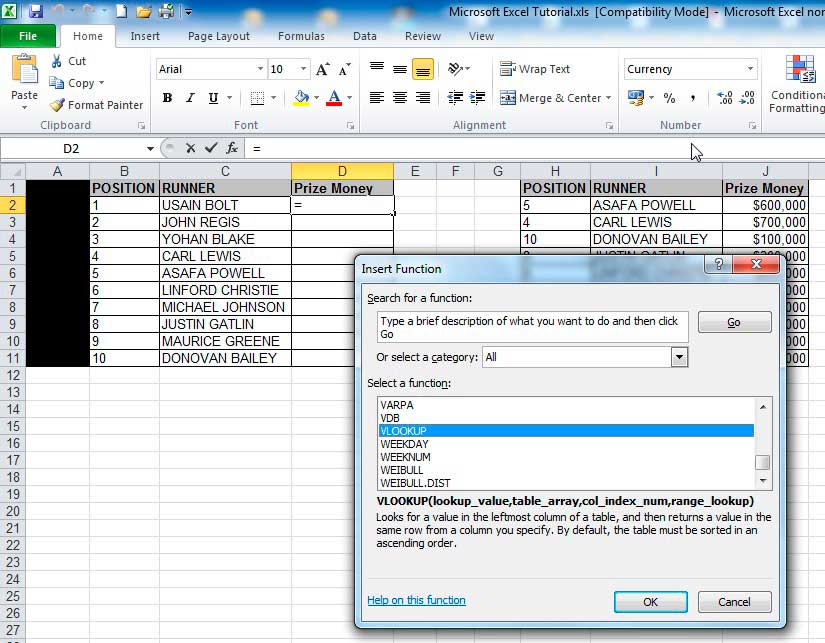
Click ‘ok’ and the function arguments window will pop up. This table will show the Syntax (a fancy word for the format of the formula) and it will display the different parts of the syntax ie
VLOOKUP(lookup_value,table_array,col_index_num,range_lookup)
STEP 3
Here, you should click into cell ‘B2’ because that’s the first number or reference for which you want to lookup a value. The ‘look up value’ is the corresponding value we want to find in the first column of the second table – so we want to find out what ‘Prize Money’ the runner in position 1 got in the table that spans columns H to J.
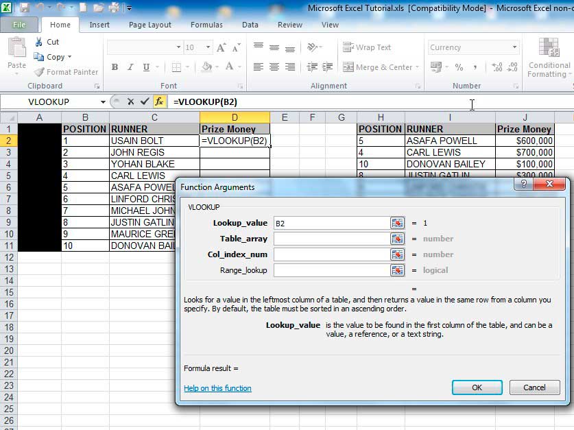
STEP 4
Now click in the next field, the ‘table array’ field (the table array consists of two or more columns of data and the first column in the table array – in this case col. H – has the corresponding numbers that the ‘lookup value is looking at ie the runner positions in this case).
STEP 5
After clicking in the ‘table array’ field, you then need to highlight the columns that that you want to look up data from; so here, we will highlight columns H to J, because our lookup value column starts from column H in the second table, and the Prize Money which we want to check is in col. J –
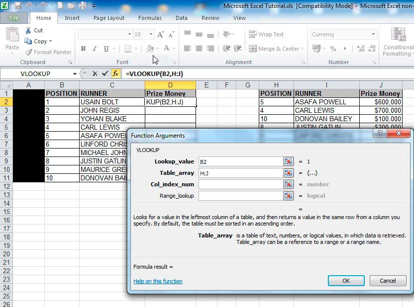
STEP 6
When you highlight the columns, you should note that column J is the 3rd column from column H. We then move onto the next step, Col_index_num, which is the column Index number. Click in that field and type the number 3) – this is because column J is three columns away from column H.

STEP 7
Now, for the last bit, simply click in the ‘range lookup’ field and type in the word false. You should always type in the word false here, because we want the vlookup to return an exact match for what we‘re looking for, and if it doesn’t then we want it to return the word false.

Now click ‘Ok’, and like magic, you will notice that the vlookup has returned the figure of $1,000,000 against Usain Bolt’s name in the first table. If you look at the second table, the figure of $1,000,000 is also against Usain Bolt’s name, so we know the vlookup has worked. And that’s how you string together the vlookup formula in excel.
Now all you have to do is drag down the formula, so that the cells below cell D2 populate, and you save yourself the hassle of manually finding the corresponding Prize Money value for each and every athlete in the first table. In a work scenario, if you had hundreds of rows of data, this would literally save you hours of work!
IMPORTANT point to note – the numbers in the “lookup value” column MUST precede the data you’re looking up! The same is true for the table that you are looking up data from (you must ALWAYS move from the left to the right, when using vlookups!)
If you have problems with your vlookup click here– 6 common problems:
We ask that you take a moment to read our Terms and Conditions and Privacy Policies.

Excel Tutorials | Learn Excel