Vlookup between two workbooks / Vlookup between multiple worksheets
Below is an example of a vlookup between two different workbooks, which a lot of you have been asking about.
To make it as easy as possible for you to understand the steps, we’ve included the two files we use for this free excel vlookup tutorial here: Workbook without prices and Workbook with prices.
You can’t learn how to drive a car by just reading a book, and for that reason, we’ve given you access to the files that we use – after all, the best way to learn is by doing! Other sites do not offer you the files, but we do. We recommend that you have both files open before you begin the tutorial.
The workbooks contain a list of products which the majority of people would buy in a supermarket – Milk, Bread, Jam, etc.
We have intentionally kept the files simple. We’re going to use the vlookup function to get the prices of the food data from the “workbook with prices” into the “workbook without prices”.
Step 1
Before you start, open both workbooks from this site AND make sure you’ve clicked the “Enable editing” button in BOTH workbooks then save them to your Desktop, otherwise any changes you make won’t work!
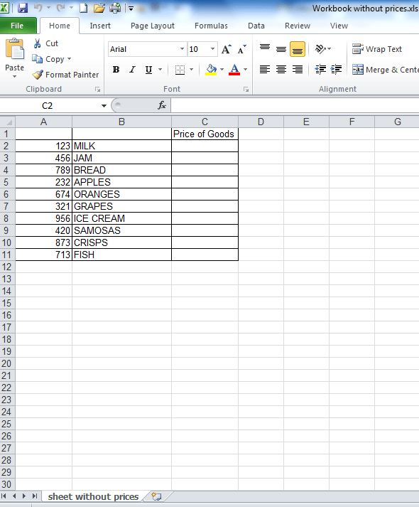
When you open the “workbook without prices” file you will see the screen below. Column C in this workbook is where we will pull in the “Price of the Goods” from the other workbook. Cell C2 in the “workbook without prices” will already be selected – if it isn’t, click in cell C2, as that’s where we want the first result to appear.
Step 2
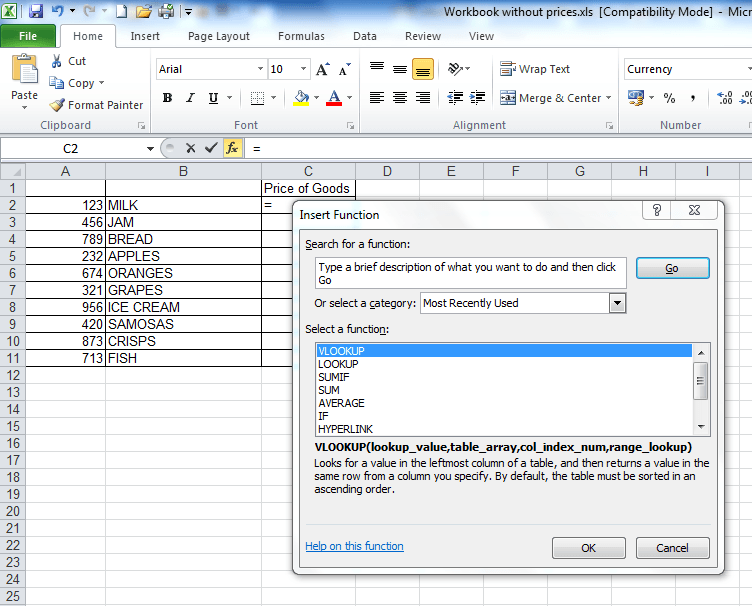
Click on the “fx” button which is just above column B (see screenshot below). The ‘Insert Function’ window will then show up (also shown in the screenshot below). If the “vlookup function” is already selected, like in the screenshot below, click “ok”.
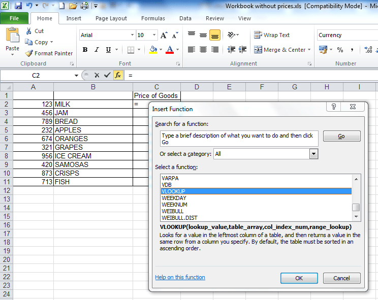
If the “vlookup function isn’t already selected, then in the “or select a category” field shown in the screenshot above, change the option in the drop-down from “most recently used” to “All” then scroll down until you get to the vlookup function, as shown in the screenshot below.
Once you’ve selected the “vlookup function” from the drop down menu and clicked ok, the “Function Arguments” window will appear.
Step 3
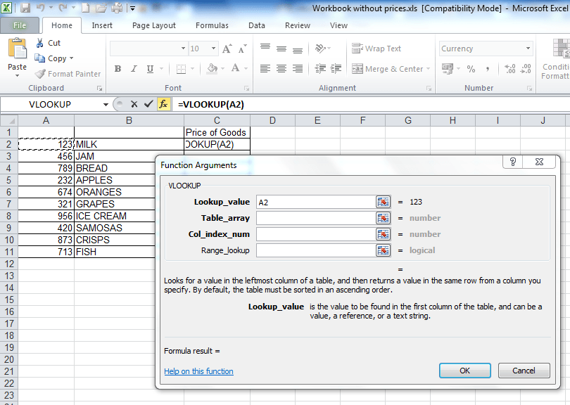
The “Function Arguments” window will show 4 different fields which need to be populated for the vlookup to work. For the first field, the “Lookup_value”, click on cell A2, as illustrated in the image below.
Step 4
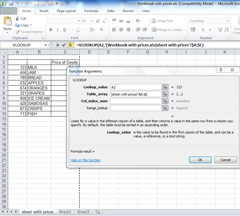
Now click into the “Table_array” field (a “table array” is a fancy phrase for describing two or more columns of data).
Step 5
This part is where the other workbook comes in! After you’ve clicked in the “Table_array” field, click into the other workbook (it’s called “workbook with prices”) and highlight columns A – C in that workbook. We highlight columns A – C in this workbook because column A has the “Lookup_value” that is in the “workbook without prices” and column C has the “Price of Goods” data that we want to extract from this workbook. When you highlighted columns A – C, you may have noticed that the characters “3C” appeared at the top of column D – this is a quick way of Excel telling you how many columns there are in the data you’ve highlighted – it saves you having to count the columns manually, which a lot of people in offices do! If you didn’t notice that, clear the data in the “table array” field and highlight columns A – C again in the “workbook with prices” – ensure you hold the mouse key as as soon as you let go, the “3C” will disappear. Many office workers don’t know this trick and waste a lot of time manually counting the columns! But we’re here to save you time!
NB – an alternative, but IMPORTANT way to populate the “Table_array” field is to highlight the range of data you’re looking up, starting with your first unique value – in this case cell A3. So you’d highlight cells A3 to C12, because C12 is the last cell in the range. You’d then need to FIX this table array by putting dollar signs in before the H, before the 2, before the J and before the 11, so your formula at the end looks like this: =VLOOKUP(B2,$A$3:$C$12,3,FALSE). If you’re in the table array field and you press F4, then Excel will do this automatically for you.This is useful to know if a spreadsheet at work doesn’t allow you to highlight columns A to C because some cells are merged or you’re getting an invalid error. But for now, just leave it, ensure, you’re fields look the same as those in the screenshot below then proceed to Step 6, the second last step.
Step 6
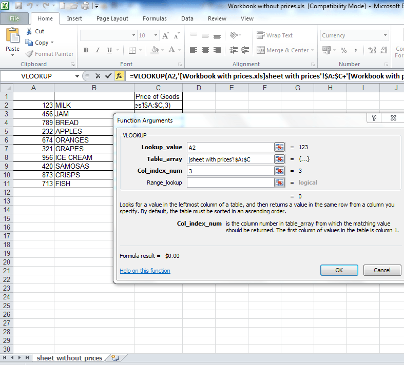
Click into the “Col_index_num” field – you will notice that your screen returns back to the first file, the “workbook without prices” – don’t panic! All you have to do here is put in the number 3. We put in the number 3 here because column C in the “workbook with prices” has the prices of the goods that we want and it is three columns away from column A, which has the unique lookup values that we are using. Or if you noticed the “3C”, it means “3 columns” so you know you have to insert the number 3 in the “Col_index_num” field. A screenshot of how everything should look so far is below.
Step 7
The final step! Click into the ‘range lookup field’ and type the word ‘FALSE’. Click ‘OK’ and, like magic, the formula will return the first result that we’re looking up. After that, simply drag down the formula in cell C2 in the “workbook without prices” and the “prices” of all the other goods in this file will auto-populate. Easy, right!? Typing the word ‘FALSE’ here will ensure that the vlookup only returns an EXACT match. If it doesn’t find an exact match for the ‘lookup value’ we’re using, then it will return an N/A – more about this in the “10 common problems” page above.
Your formula in the end should look like this (in cell C2 in the workbook without prices): =VLOOKUP(A2,'[Workbook-with-prices.xls]Sheet1′!$A:$C,3,FALSE)
If your formula does not look like this, then you need to check that you’ve followed the steps above correctly.
3 people said they couldn’t get to the second workbook in step 5. This is because they hadn’t clicked on the ‘enable editing’ button shown in the screenshots at the beginning of this tutorial in BOTH workbooks! Please make sure you do this if this problem applied to you, before posting a comment. In fact, you should ALWAYS click ‘enable editing’ if you’re using formulas in Excel. It’s good practise and will help you.
If you want to learn about Pivot Tables, you can do so via this website we created following user demand: http://pivottablesinexcel.com/
If you have problems with your vlookup click here – 13 common problems:
We ask that you take a moment to read our Terms and Conditions and Privacy Policies.

thanks heaps! helped me big time, keep doing what you guys are doing.
what if i want to copy 2 columns of data from one workbook to another??
Just do two vlookups.
Thanx….i work in back-office and this tutorial really helped me, thank you so much
great help indeed
Great Tutorial.
Is there a way for this to work without having the source workbook open?
Thanks,
No – you need the sourcebook open when you’re first creating the formula, after which you can close it and forget about it (but not delete it! Otherwise you’ll get the #REF error described on this page: https://howtovlookupinexcel.com/10-common-problems-with-vlookups)
I have on sheet that has 1000 names and one that only has 200. i am doing my vlookup on the 1000 name sheet against the 200. i know my formula is correct but not all are showing up
Hi Daniel
If they’re not showing up in the 1000 name sheet and they definitely exist in the 200 sheet, then there’s an error with your formula. If the info isn’t confidential, send it to the email address that you get this update from and I’ll have a look.
Awesome tips! You are amazing!
Thank you.
I have two workbooks. The first workbook (A) is a master worksheet with 5000 names, first and last name, email and telephone numbers in separate columns. The second worksheet (B) is just a list of people by first and last name who have attended a party. I am using vlookup to find people listed in workbook B to see if they are listed in workbook A. I they are listed in workbook A I pull the email address and telephone numbers over to workbook B. My problem is looking for a person with the last name of Brown but there are 8 people with the same last name Brown in workbook A. So need to check first name too. I cannot figure the right formula do do that. I have sample workbooks to try testing vlookup and the and function but its stll not working. Any help available to come up with the correct formula to do this?
Yes. If you had the name “John” in cell A1 and the surname “Brown” in cell B1, you’d need to put the formula =A1&B1 in cell C1, which would combine the first name and surname, and therefore give you a “unique” party goer!
This would make John Brown become JohnBrown (with no space between first and last name).
You’d just then need to drag this formula down for all the other names and use the name in column C to do the vlookup, as Sharon Brown would be SharonBrown (with no space) which is obviously different to JohnBrown. Let me know if you need further clarification.
Gr8 Explanation!! Thank you guys 🙂
Thanks!
Is cell C2 supposed to have $1.44 by the end?
Yes – you can see that Milk in the other workbookbook has a price of $1.44.
We have three workbooks that we have linked using VLOOKUP, but we keep losing the “LINK”.
It is on the server as Z:\Public….
Often, we open the workbook and the VLOOKUP is reading Y:\Public
We still have data even though there is no such folder as Y:\Public, but the data is no updated to the Z:\Public file.
HELP???
Thanks!
Hi Ken
That’s a bizarre problem. Sounds like the files are being moved around by your IT colleagues, as they can manage the location of files and folders and I’ve encountered situations where they archived documents and moved files without telling me!
I’d suggest adding the data from the workbooks you’re looking up into separate SHEETS in the workbook where you’re gathering all the data. This will ensure that everything is in one file / workbook and even if other workbooks are tampered with, the data you need is in the one workbook, but in separate sheets.
Hope that helps.
Thanks. Really Helpful
You’re welcome.
Thanks, now i understood vlookup.
Very Nice tutorial, now i understand vlookup.
Thanks a lot.
It is an awesome tutorial. Thanks a lot. Its very easy to understand.it helped me a lot.
Hi,
That was awesome actually. Can you tell me how to handle duplicates.
I have 3 rows in my sheet 1 (A, A, B) and i have 2 rows in my sheet 2 (A,B). How do i get the values for both the values of sheet 1 in sheet 2.
Thanks,
Sudheer
If you have duplicates, you should remove them from the source data.
The vlookup will only return the first record it comes across for the unique value you’re using to search for records. Eg if you had Usain Bolt in sheet 1 and you had another sheet (sheet 2) which had the times that Usain Bolt ran in one race, the vlookup would return the first result it came across for Usain Bolt in sheet 2, using the method I’ve described in the tutorial. All the other results would be ignored – this is explained further in problem number 4 on this page:https://howtovlookupinexcel.com/7-common-problems-with-vlookups
You’d obviously need to work out why you have duplicates in the first place and ensure you’re referencing the latest / correct data in your spreadsheet. Once you know why, there is a button for removing duplicates in Excel 2007 onwards which will help with the duplicate removal.
Thats awesome, you made it so simple to understand Thanks Alot!!!!
You’re welcome.
Super hit,extremely valuable best job
Thanks
Hi Admin,
just wanted to say thank you so much!
i have been having so much trouble with this for so long i was ready to give up. so thank you for helping me i now understand what i was doing wrong and it is working on my own file! so thank you again 🙂
No worries – glad I was able to help!
The Vlookup is not working. Is it because I have numbers and letters in one field? What should I store the number as…a number or text, general?
Hi Jess
The format to store your number in will depend on how you present the data.
If you send me the file (which I presume you downloaded from this site), I’ll look into the error.
Hi admin,
First of all thank you for tutorial which is very helpful.
I have another question, i have two files on the network but on different sharedrives. When i use this formula in e.g. Share Drive Z:\Overtime sheet (to get employees data) from the data base from Share Drive Y:\Employee Data. It gives me the output from row 6000 onwards. Whereas I have data from A1:X1 to A7000 to X7000.
Could you please support on this?
Thanks,
Hi Kashif
Can you send me the formula you used for your spreadsheet?
You guys rockx,tutorial is easy and informative,many thanks to you people 😀
Thank YOU A+
Awesome! Thanks.
Thanks, It was really helpful.
Thanks Sabuj.
Thank U So Much..
I found your tutorial very useful.
Thnxs lott, it solved my prblm
Thank you for making this so easy to learn! Much appreciated!
Great tutorial on V-lookups! I am having a problem with using V-lookups when trying to compare two sheets that may have similar information. for example: John doe on sheet1 and I want to see if John doe is on sheet 2… when i use the v-lookup function its just returning #N/A? could you help with this?
Hi Ben
There’s lots of demand for solutions to different problems. Just finished a pivot tables tutorial. I’ll post something on your query in the next few weeks.
Thank you so much…. 🙂
To be honest, u saved my job, so again, thank you.
When r v going to hv a tutorial on hlookup & pivot?
Love and regards
Hi Kaushik
Thank you.
A pivot table tutorial should be available by the end of next week. Will let you know if not.
Here I need a clarification. I have two work books having the same data but one is having more and its not in order like. Now I want to check whether the data in one workbook is existing in another workbook. Could u pls help me out of this as this is most usefull to me in work.
Hi
The solution to that question is a bit long winded, but I am planning to put it in an ebook that should be available in about a month or so.
Such a wonderful guidance of Vlookup.
Very helpful.
Thank you. This was a really nice and simple explanation. Please make a tutorial for hlookup also.
Thanks Eldorado – will look into doing a tutorial for the hlookup in future.
awesome it is really usefully…..very easy to understand…i was trying to understand vlookup between two workbooks but finally i followed all ur steps and i got it applying same to hlookup…pls help in macros…….thank q so much………
Hi Sunita
Just finished material on Pivot Tables (http://pivottablesinexcel.com/). I will look into doing something on macros in future.
ooooooooooo thank q dear……….waitng for macros…..and one more question…to become expert in excel what r d topics i need to cover n practice……
Hi Sunita
Just to manage your expectations, there is another site I’m working on, so macros content may not be available for a while.
There are many functions that you need to become an expert, but they all depend on the job you do. vlookups, are of course, very useful, along with IF statements, pivot tables (for which I’ve created a tutorial here: http://pivottablesinexcel.com/) and other functions. But it depends on the job you’re doing.
Thanx u made it so easy
These are all terrific examples – I have been struggling to put together SIMPLE samples for our 10 offices (mostly non users). You have saved me quite a bit of work!
Thanks.
Thanks for making Vlookup so easy and simple to understand! KUDOS!!
Thanks dude.
YOU KNOW, MY ENDURANCE IS NOT ENOUGH TO WORK ON THIS COMMAND. IN ALL CELLS, IT SHOW N/A. I COULDN’T CORRECT THEM.
PLEASE ADVISE ME
Hi Dani
I’ve dumbed down the explanation as much as possible. If you still don’t get it, I’d suggest that you start with the tutorial on this page, which has the explanation all on one spreadsheet: https://howtovlookupinexcel.com/ (this directs you to the 2010/2007 tutorial on one spreadsheet). If you follow the instructions properly, it will work.
Thanks a lot bro. it really helped me a lot.
No worries.
what a nice vlookupcode
After going through your guide Vlookup is now a piece of cake…Thanks a million times 🙂
You’re welcome.